Experimental Markets Chris Starmer TSU Short Course in


![Not Necessarily • “The mere fact that […] supply and demand schedules exist in Not Necessarily • “The mere fact that […] supply and demand schedules exist in](https://slidetodoc.com/presentation_image_h/0e16512f97007216f30f87b8cfefcfc9/image-17.jpg)

- Slides: 71

Experimental Markets Chris Starmer TSU Short Course in Experimental and Behavioural Economics, 5 -9 November 2012

Background • In 2002, Vernon L. Smith Shared Nobel prize in Economic Science • For work developing experimental approaches to study of markets – Discovery of remarkable properties • This (more-or-less) started of one of the major research programmes in experimental econ. • I talk about this today Visit - www. nobelprize. org/nobel_prizes/economics/laureates/

Route Map The approach Smith pioneered uses an experimental technique called Induced Value Methodology A technique for setting up experimental markets Today I will Introduce the method Show some classic – often replicated - results (performance of competitive equilibrium) Extension to asset markets

What is an Experimental Market? • Experiment in which: – Some experimental subjects assigned roles of buyers and/or sellers – There are ‘goods’ that can be traded • Often ‘induced value’ tokens (See later) • Markets (usually) set up so that: – there are potential gains from trade • Experimenter controls rules of trade • Observes what happens

V. Smith 1989, J. Econ. Perspectives • Market experiment is conjunction of: – Environment • Participants, endowments, preferences… – Institution • Rules of trade, who can do what, when …. . – Behaviour • Experiments often involve – Creation/manipulation of Environ/Institution – With view to observing consequent behaviour

A Classic Market Experiment Vernon Smith (1962) J. Pol. Econ. “An Experimental Study of Competitive Market Behaviour”

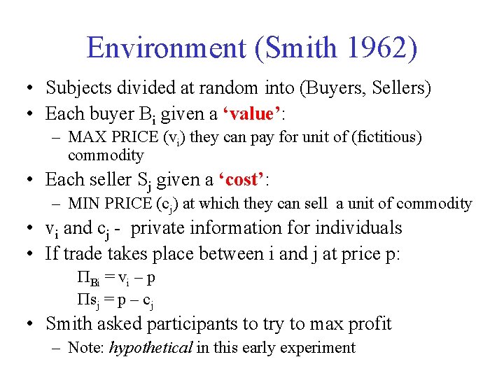
Environment (Smith 1962) • Subjects divided at random into (Buyers, Sellers) • Each buyer Bi given a ‘value’: – MAX PRICE (vi) they can pay for unit of (fictitious) commodity • Each seller Sj given a ‘cost’: – MIN PRICE (cj) at which they can sell a unit of commodity • vi and cj - private information for individuals • If trade takes place between i and j at price p: Bi = vi – p sj = p – cj • Smith asked participants to try to max profit – Note: hypothetical in this early experiment

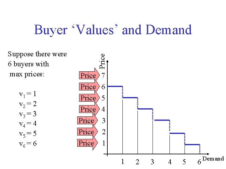
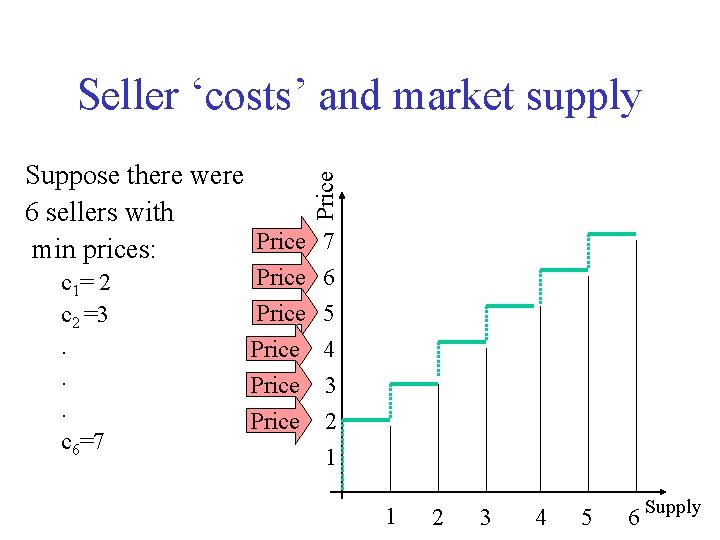
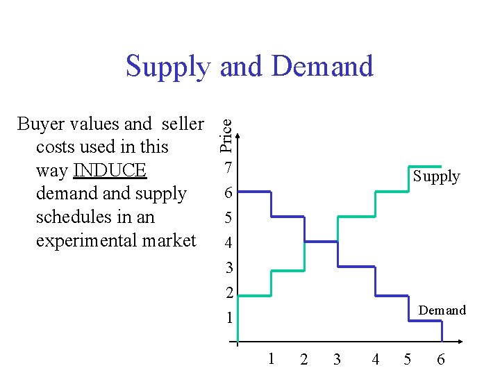
Interpretation of Payoffs • In the aggregate: – the values given to buyers define a demand function – so, for any potential price, the values determine the maximum quantity that can could be purchased Illustration. . . .

Suppose there were 6 buyers with max prices: v 1 = 1 v 2 = 2 v 3 = 3 v 4 = 4 v 5 = 5 v 6 = 6 Price Buyer ‘Values’ and Demand Price 7 Price 6 Price 5 Price 4 Price 3 Price 2 Price 1 1 2 3 4 5 6 Demand

Seller ‘costs’ and market supply Price Suppose there were 6 sellers with Price 7 min prices: c 1= 2 c 2 =3. . . c 6=7 Price Price 6 5 4 3 2 1 1 2 3 4 5 6 Supply

Buyer values and seller costs used in this way INDUCE demand supply schedules in an experimental market Price Supply and Demand 7 6 5 4 3 2 1 Supply Demand 1 2 3 4 5 6

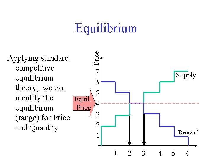
Price Equilibrium Applying standard competitive 7 equilibrium 6 theory, we can 5 identify the Equil. 4 Price equilibirum 3 (range) for Price 2 and Quantity Supply Demand 1 1 2 3 4 5 6

Back to Smith 1962…. .

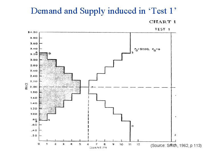
Supply and Demand conditions in Smith 1962 • Smith reports results of running several market sessions • Demand Supply conditions vary • Here are D and S schedules from one market

Demand Supply induced in ‘Test 1’ (Source: Smith, 1962, p 113)

Question Should we expect equilibrium in this experimental market?
![Not Necessarily The mere fact that supply and demand schedules exist in Not Necessarily • “The mere fact that […] supply and demand schedules exist in](https://slidetodoc.com/presentation_image_h/0e16512f97007216f30f87b8cfefcfc9/image-17.jpg)
Not Necessarily • “The mere fact that […] supply and demand schedules exist in the background of a market does not guarantee that any meaningful relationship exists between those schedules and what is observed in the market they are presumed to represent. All the supply and demand schedules can do is set broad limits on the behaviour of the market. • (Vernon Smith, 1962, p. 115) • In other words, D and S determine the set of feasible trades • What will arise as the actual pattern of trading is an open question

Institutions Matter • Simple thought experiment demonstrates that institutions matter…. • Consider an extreme case where the rules of the experiment are – Everyone sits in isolation – No possibility to communicate with other potential traders • In this case, the institutional arrangements inhibit/prevent trade: – No prices formed – Zero quantity traded

Smith’s 1962: uses a ‘Double Auction’ • Sequence of trading periods (5– 10 mins) • Experimenter opens/closes trading periods • At any time during trading period B (or S) are free to make verbal offers (hence DA) – These must respect max values (min costs) • Improvement rule for new offers – Higher bid/lower offer than current best • Any S ( or B) can accept an existing offer to buy (or sell) s. t. cost (value) constraints • Acceptances result in binding contracts – B/S pair drop out of market once party to a contract • Trading period continues until no further contracts are being made

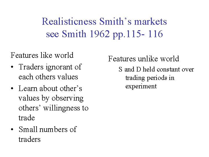
Realisticness Smith’s markets see Smith 1962 pp. 115 - 116 Features like world • Traders ignorant of each others values • Learn about other’s values by observing others’ willingness to trade • Small numbers of traders Features unlike world S and D held constant over trading periods in experiment

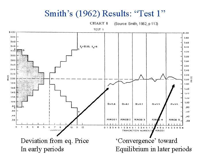
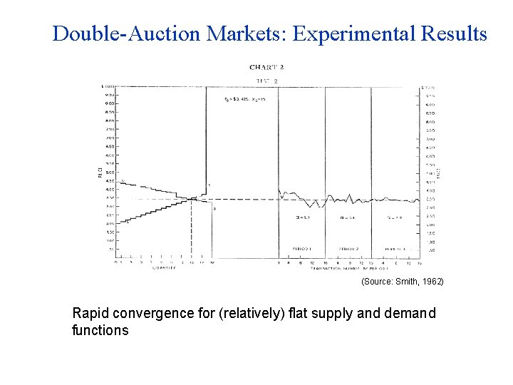
Smith’s (1962) Results: “Test 1” (Source: Smith, 1962, p 113) Deviation from eq. Price In early periods ‘Convergence’ toward Equilibrium in later periods

Variation in S and D Schedules 1. Changing slopes of Demand Supply functions

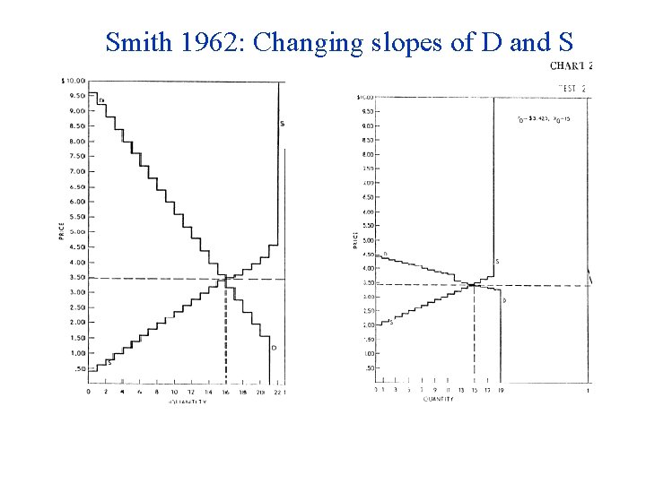
Smith 1962: Changing slopes of D and S

Double-Auction Markets: Experimental Results (Source: Smith, 1962) Rapid convergence for (relatively) flat supply and demand functions

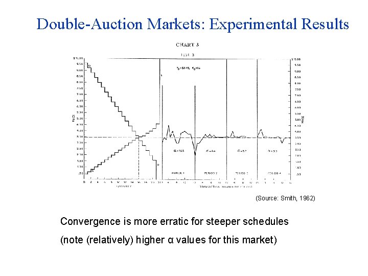
Double-Auction Markets: Experimental Results (Source: Smith, 1962) Convergence is more erratic for steeper schedules (note (relatively) higher α values for this market)

Impact of Surplus Distribution

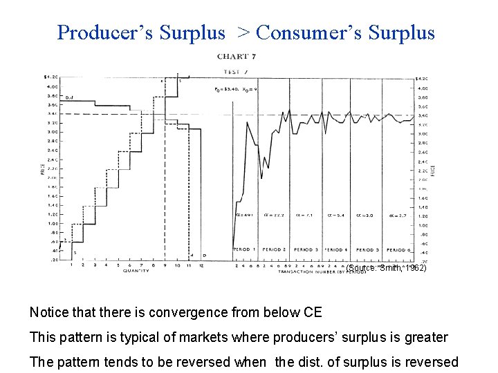
Producer’s Surplus > Consumer’s Surplus (Source: Smith, 1962) Notice that there is convergence from below CE This pattern is typical of markets where producers’ surplus is greater The pattern tends to be reversed when the dist. of surplus is reversed

Variation in S and D Schedules Demand Expansion

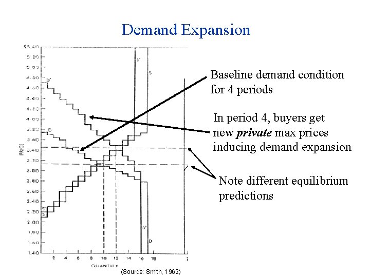
Demand Expansion Baseline demand condition for 4 periods In period 4, buyers get new private max prices inducing demand expansion Note different equilibrium predictions (Source: Smith, 1962)

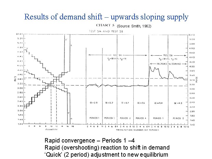
Results of demand shift – upwards sloping supply (Source: Smith, 1962) Rapid convergence – Periods 1 – 4 Rapid (overshooting) reaction to shift in demand ‘Quick’ (2 period) adjustment to new equilibrium

Surprised by convergence in Smith’s experiment?

Perhaps you should be? • Consider some of key assumptions of CE models – – Many Buyers Many Sellers Price Taking Perfect Info • Compare with Smith’s markets – Handful of traders – Price Making – Imperfect info Each trader knows only their own value. Individuals do not know the general supply and demand conditions

Commenting, years later on accumulated evidence from experiments using DA markets, Smith argues…. • “There are no experimental results more important or more significant than that the information specifications of traditional competitive price theory are grossly overstated. The experimental facts are that no double auction trader needs to know anything about the valuation conditions of other traders, or have any understanding or knowledge of market supply and demand conditions, or have any trading experience (although experience may speed convergence) or satisfy the quaint and irrelevant requirement of being a price ‘taker’ (every trader is a price maker in a double auction). ” – Vernon Smith (Quote reproduced in Holt, p 370)

Session 5 – Part II Asset Market Experiments

Asset Markets I discuss application of induced value to study asset markets. I discuss a landmark study Plott, C and S. Sunder (1982) – “Efficiency of Experimental Security Markets with Insider Information…. . ”, J. Political Econ. • And some subsequent literature

Characteristics of Asset Markets • ‘Assets’ – Value may depend on uncertain state of nature – May deliver multi-period returns (dividends) • Experimental assets typically have one or both of these features • Traders – buy and sell with view to profit – potential for ‘speculation’ • Often asymmetric information – ‘Insiders’ know more about value of asset (or state of nature)

Two (caricatured) views on efficiency of asset markets Label these loosely as: The efficient market hypothesis The speculation hypothesis

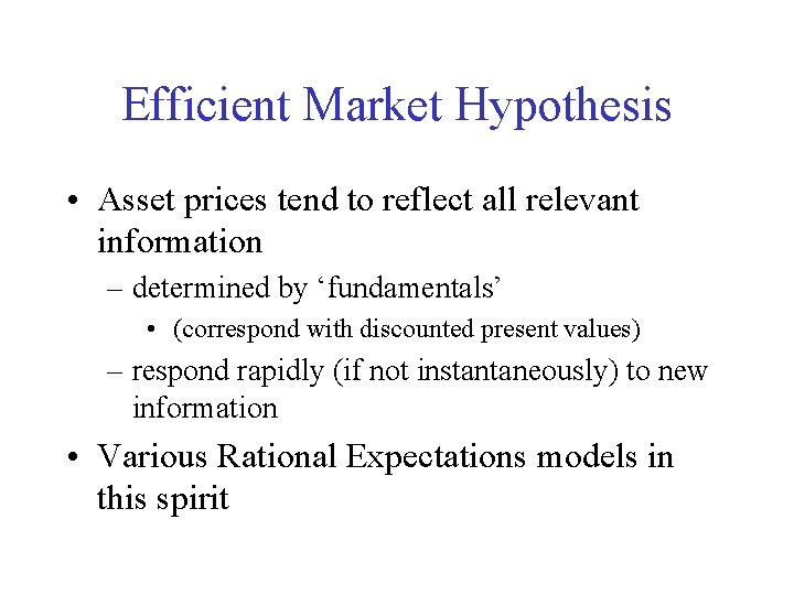
Efficient Market Hypothesis • Asset prices tend to reflect all relevant information – determined by ‘fundamentals’ • (correspond with discounted present values) – respond rapidly (if not instantaneously) to new information • Various Rational Expectations models in this spirit

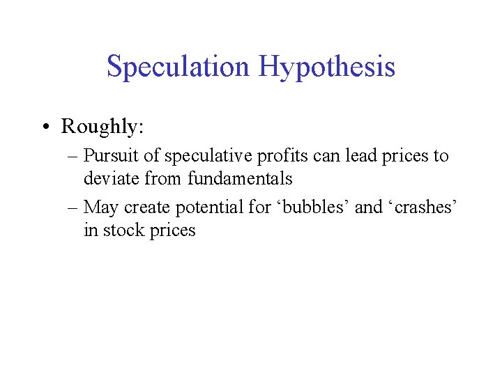
Speculation Hypothesis • Roughly: – Pursuit of speculative profits can lead prices to deviate from fundamentals – May create potential for ‘bubbles’ and ‘crashes’ in stock prices

One rationale for asset market experiments • EMH is difficult to test with field data: – Researchers don’t know discounted PVs – Researchers don’t know what relevant info is – Researchers can observe if responses to good and bad news have right sign, but don’t know if price levels reflect fundamentals

Advantage of Experiments In principle, Experimenter can: • control fundamentals – e. g. implement asset with PV known to experimenter • implement markets with Rational Expectations Equilibria known to experimenter • manipulate information structures – E. g. create insider information and observe impact

Issues • Two what extent, and under what conditions, do markets: – disseminate and aggregate dispersed information? – achieve rational expectations equilibria? • To what extent, and under what conditions, do we see out of equilibrium phenomena? – e. g. speculative bubbles and crashes

A Classic Asset Market Experiment Plott and Sunder 1982

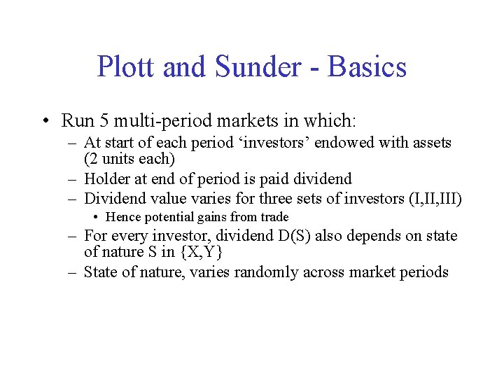
Plott and Sunder - Basics • Run 5 multi-period markets in which: – At start of each period ‘investors’ endowed with assets (2 units each) – Holder at end of period is paid dividend – Dividend value varies for three sets of investors (I, III) • Hence potential gains from trade – For every investor, dividend D(S) also depends on state of nature S in {X, Y} – State of nature, varies randomly across market periods

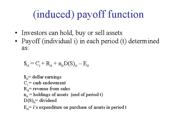
(induced) payoff function • Investors can hold, buy or sell assets • Payoff (individual i) in each period (t) determined as: $it = Ci + Rit + nit. D(S)it – Eit $it= dollar earnings Ci = cash endowment Rit= revenue from sales nit = holdings of assets (end of period t) D(S)it= dividend Eit= i’s expenditure on purchase of assets in period t

state of nature • Determined randomly in each period (‘year’) • All agents knew: – State probabilities (via training

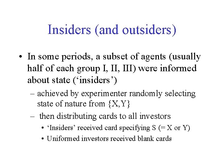
Insiders (and outsiders) • In some periods, a subset of agents (usually half of each group I, III) were informed about state (‘insiders’) – achieved by experimenter randomly selecting state of nature from {X, Y} – then distributing cards to all investors • ‘Insiders’ received card specifying S (= X or Y) • Uniformed investors received blank cards

P+S: Predictions Consider two theoretical models Private Information (PI) Rational Expectations (RE) Common assumptions: Agents are risk neutral & follow simple decision rule: – Buy assets if P < E(dividend) – Sell assets if P > E(dividend) PI: E(. ) based on private information Hence different E(. ) for Insiders/Outsiders RE: E(. ) based on full information Market behaves as if all agents know realised state

PI and RE Lead to different predictions re: –Market prices –Pattern of asset holdings Illustrate with P + S: “Market 3”

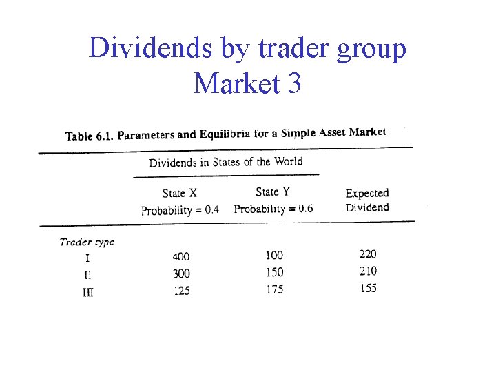
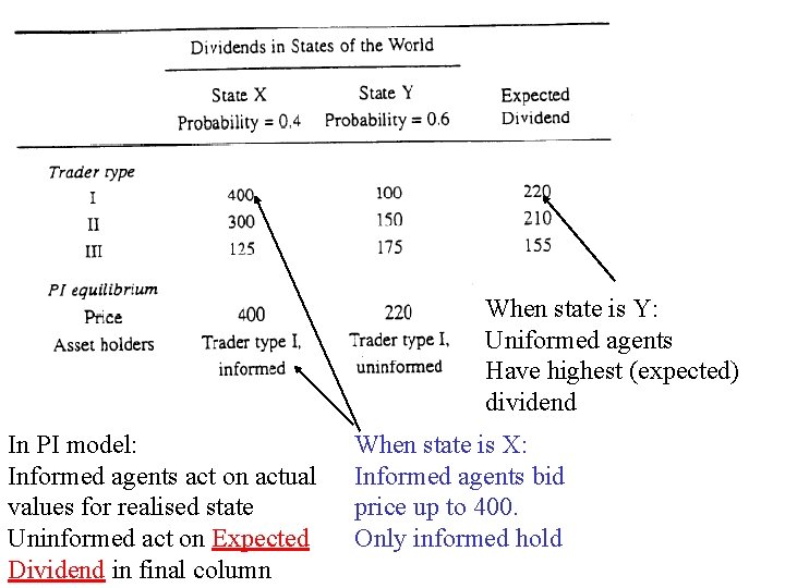
Dividends by trader group Market 3

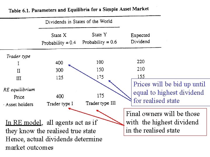
Prices will be bid up until equal to highest dividend for realised state In RE model, all agents act as if they know the realised true state Hence, actual dividends determine market outcomes Final owners will be those with the highest dividend in the realised state

When state is Y: Uniformed agents Have highest (expected) dividend In PI model: Informed agents act on actual values for realised state Uninformed act on Expected Dividend in final column When state is X: Informed agents bid price up to 400. Only informed hold

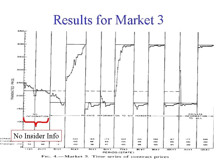
Results for Market 3 No Insider Info

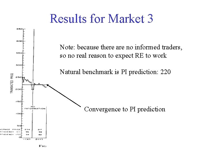
Results for Market 3 Note: because there are no informed traders, so no real reason to expect RE to work Natural benchmark is PI prediction: 220 Convergence to PI prediction

Periods 3 – 10 half traders are informed

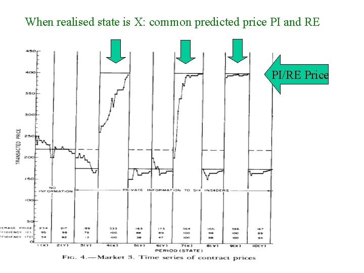
When realised state is X: common predicted price PI and RE PI/RE Price

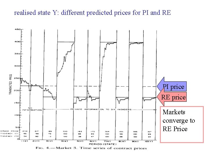
realised state Y: different predicted prices for PI and RE PI price RE price Markets converge to RE Price

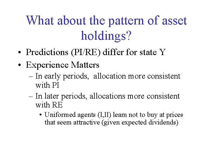
What about the pattern of asset holdings? • Predictions (PI/RE) differ for state Y • Experience Matters – In early periods, allocation more consistent with PI – In later periods, allocations more consistent with RE • Uniformed agents (I, II) learn not to buy at prices that seem attractive (given expected dividends)

P + S Conclusions • “Given time and replication these markets behave substantially as predicted by RE equilibrium models. There seems to be no doubt that variables endogenous to the operation of these markets served to convey accurately the state of nature to otherwise uninformed agents. We can conclude that the RE models must be taken seriously as not universally misleading about the nature of human capabilities and markets” p 692

Later Research • Later research – explores factors affecting efficiency of info transmission – Balance of informed vs uninformed – Uncertainty re presence of informed – When state of nature is revealed – Experience of traders – Number and Nature of assets traded

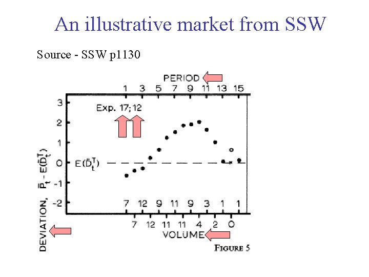
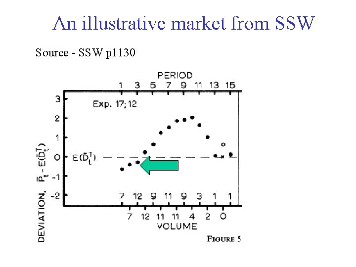
Hunting Bubbles • Smith, Suchanek and Williams 1988 (“SSW”) – “Bubbles crashes and endogenous expectations in experimental spot asset markets”, Econometrica, 56, 1119– 51.

Why Hunt Bubbles? • SSW conjecture that real asset markets may be prone to bubbles defined as: – “trade in high volumes at prices that are considerably at variance from intrinsic values” p 831. • But - unclear how common bubbles are in actual markets – Because we don’t know intrinsic values

SSW Design Two key distinguishing features compared to earlier asset market studies. – (eg. Plott and Sunder, 1982) • Longer lived assets – To allow ‘room’ for speculation • Induce identical dividend structures across market participants - Only obvious motive for trade is speculative

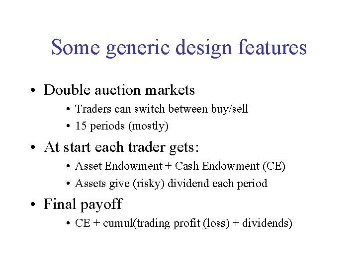
Some generic design features • Double auction markets • Traders can switch between buy/sell • 15 periods (mostly) • At start each trader gets: • Asset Endowment + Cash Endowment (CE) • Assets give (risky) dividend each period • Final payoff • CE + cumul(trading profit (loss) + dividends)

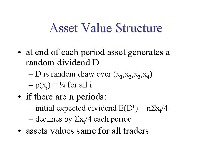
Asset Value Structure • at end of each period asset generates a random dividend D – D is random draw over (x 1, x 2, x 3, x 4) – p(xi) = ¼ for all i • if there are n periods: – initial expected dividend E(D 1) = n xi/4 – declines by xi/4 each period • assets values same for all traders

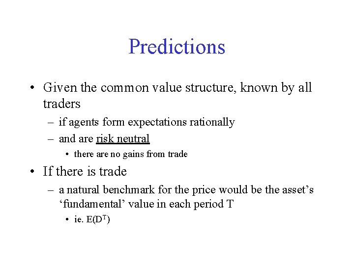
Predictions • Given the common value structure, known by all traders – if agents form expectations rationally – and are risk neutral • there are no gains from trade • If there is trade – a natural benchmark for the price would be the asset’s ‘fundamental’ value in each period T • ie. E(DT)

Some stylised results 1. Typically high volume trading 2. Price bubbles and crashes are common

An illustrative market from SSW Source - SSW p 1130

An illustrative market from SSW Source - SSW p 1130

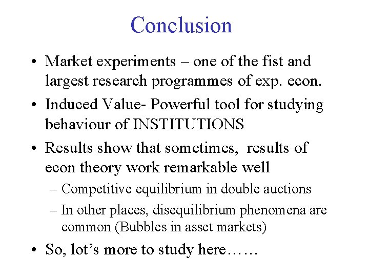
Conclusion • Market experiments – one of the fist and largest research programmes of exp. econ. • Induced Value- Powerful tool for studying behaviour of INSTITUTIONS • Results show that sometimes, results of econ theory work remarkable well – Competitive equilibrium in double auctions – In other places, disequilibrium phenomena are common (Bubbles in asset markets) • So, lot’s more to study here……

But for now, that’s all from me so Didi madloba da nakhvamdis!