Rutgers University School of Engineering Spring 2015 14

Rutgers University School of Engineering Spring 2015 14: 440: 127 - Introduction to Computers for Engineers Sophocles J. Orfanidis ECE Department orfanidi@ece. rutgers. edu Week 9 - Review Examples for Weeks 5 -8

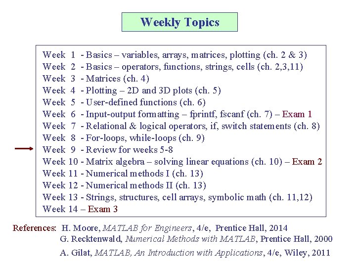
Weekly Topics Week 1 - Basics – variables, arrays, matrices, plotting (ch. 2 & 3) Week 2 - Basics – operators, functions, strings, cells (ch. 2, 3, 11) Week 3 - Matrices (ch. 4) Week 4 - Plotting – 2 D and 3 D plots (ch. 5) Week 5 - User-defined functions (ch. 6) Week 6 - Input-output formatting – fprintf, fscanf (ch. 7) – Exam 1 Week 7 - Relational & logical operators, if, switch statements (ch. 8) Week 8 - For-loops, while-loops (ch. 9) Week 9 - Review for weeks 5 -8 Week 10 - Matrix algebra – solving linear equations (ch. 10) – Exam 2 Week 11 - Numerical methods I (ch. 13) Week 12 - Numerical methods II (ch. 13) Week 13 - Strings, structures, cell arrays, symbolic math (ch. 11, 12) Week 14 – Exam 3 References: H. Moore, MATLAB for Engineers, 4/e, Prentice Hall, 2014 G. Recktenwald, Numerical Methods with MATLAB, Prentice Hall, 2000 A. Gilat, MATLAB, An Introduction with Applications, 4/e, Wiley, 2011

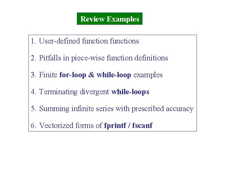
Review Examples 1. User-defined functions 2. Pitfalls in piece-wise function definitions 3. Finite for-loop & while-loop examples 4. Terminating divergent while-loops 5. Summing infinite series with prescribed accuracy 6. Vectorized forms of fprintf / fscanf

Example 1: User-defined functions function handle M-file: fmaxbnd. m function [xmax, fmax] = fmaxbnd(f, a, b) [xmax, fmax] = fminbnd(@(x) -f(x), a, b); fmax = -fmax; M-file: xsin. m function y = xsin(x) y = x. *sin(x); anonymous definition f = @(x) x. *sin(x);

[xmax, fmax] = fmaxbnd(@xsin, 0, 3); [xmax, fmax] = fmaxbnd(f, 0, 3); x = linspace(0, 3, 301); y = xsin(x); plot(x, y, 'b', xmax, fmax, 'ro'); [xmax, fmax] ans = 2. 0288 1. 8197

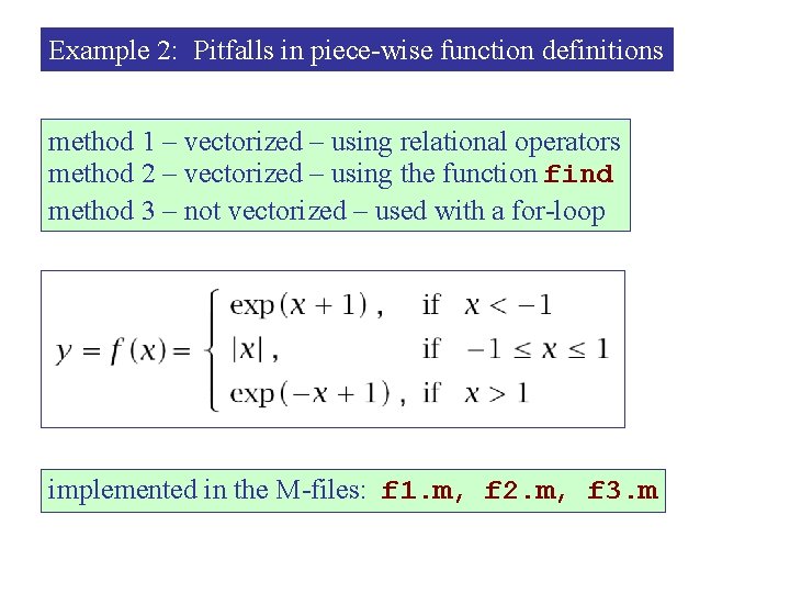
Example 2: Pitfalls in piece-wise function definitions method 1 – vectorized – using relational operators method 2 – vectorized – using the function find method 3 – not vectorized – used with a for-loop implemented in the M-files: f 1. m, f 2. m, f 3. m

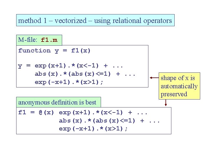
method 1 – vectorized – using relational operators M-file: f 1. m function y = f 1(x) y = exp(x+1). *(x<-1) +. . . abs(x). *(abs(x)<=1) +. . . exp(-x+1). *(x>1); anonymous definition is best f 1 = @(x) exp(x+1). *(x<-1) +. . . abs(x). *(abs(x)<=1) +. . . exp(-x+1). *(x>1); shape of x is automatically preserved

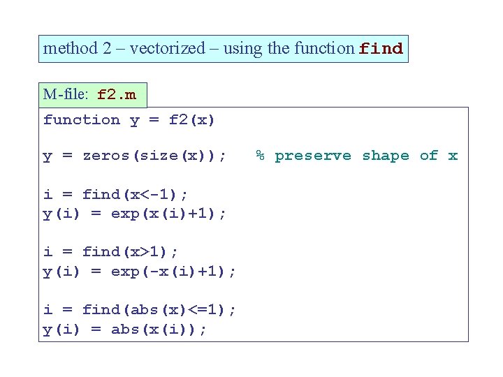
method 2 – vectorized – using the function find M-file: f 2. m function y = f 2(x) y = zeros(size(x)); i = find(x<-1); y(i) = exp(x(i)+1); i = find(x>1); y(i) = exp(-x(i)+1); i = find(abs(x)<=1); y(i) = abs(x(i)); % preserve shape of x

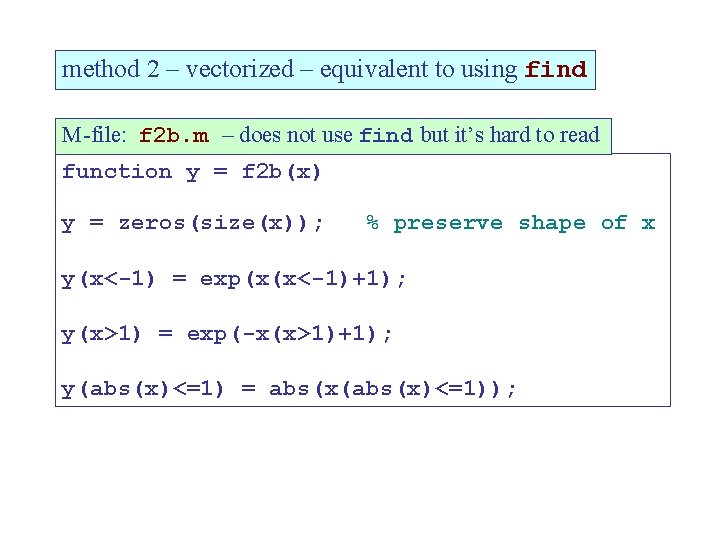
method 2 – vectorized – equivalent to using find M-file: f 2 b. m – does not use find but it’s hard to read function y = f 2 b(x) y = zeros(size(x)); % preserve shape of x y(x<-1) = exp(x(x<-1)+1); y(x>1) = exp(-x(x>1)+1); y(abs(x)<=1) = abs(x(abs(x)<=1));

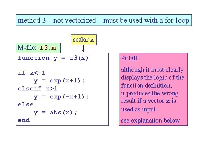
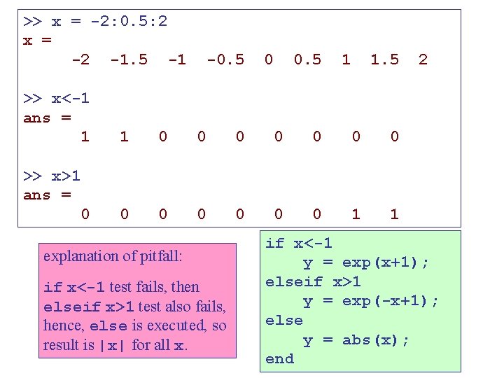
method 3 – not vectorized – must be used with a for-loop scalar x M-file: f 3. m function y = f 3(x) if x<-1 y = exp(x+1); elseif x>1 y = exp(-x+1); else y = abs(x); end Pitfall: although it most clearly displays the logic of the function definition, it produces the wrong result if a vector x is used as input see explanation below

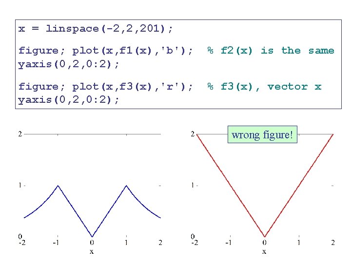
x = linspace(-2, 2, 201); figure; plot(x, f 1(x), 'b'); yaxis(0, 2, 0: 2); % f 2(x) is the same figure; plot(x, f 3(x), 'r'); yaxis(0, 2, 0: 2); % f 3(x), vector x wrong figure!

>> x = -2: 0. 5: 2 x = -2 -1. 5 -1 >> x<-1 ans = 1 -0. 5 0 0. 5 1 1. 5 1 0 0 0 0 1 1 2 >> x>1 ans = 0 explanation of pitfall: if x<-1 test fails, then elseif x>1 test also fails, hence, else is executed, so result is |x| for all x. if x<-1 y = exp(x+1); elseif x>1 y = exp(-x+1); else y = abs(x); end

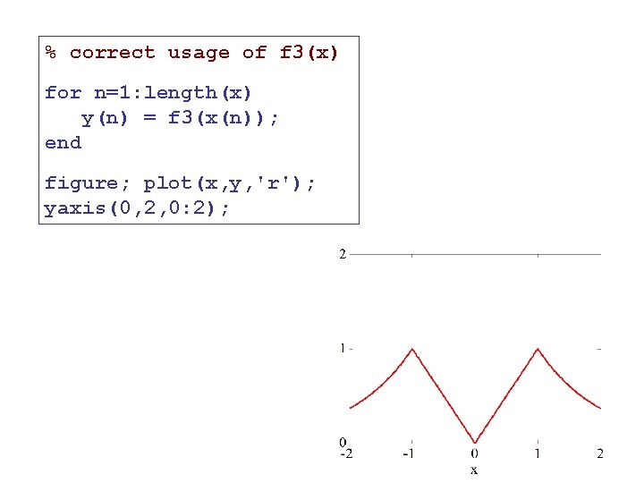
% correct usage of f 3(x) for n=1: length(x) y(n) = f 3(x(n)); end figure; plot(x, y, 'r'); yaxis(0, 2, 0: 2);

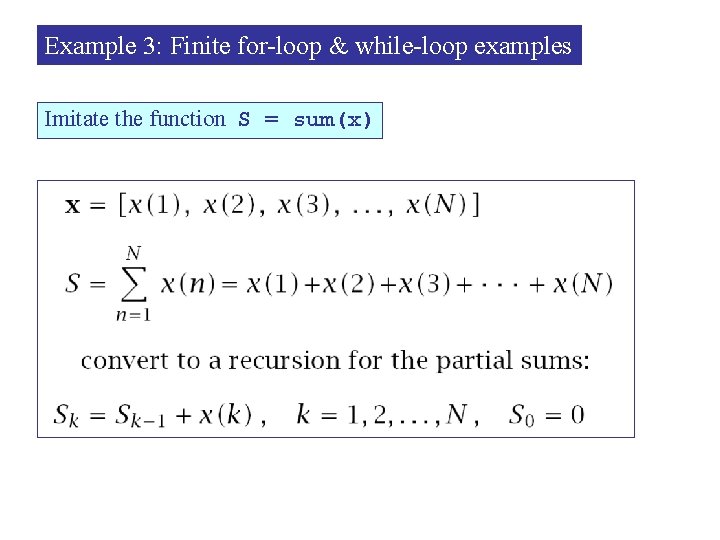
Example 3: Finite for-loop & while-loop examples Imitate the function S = sum(x)

x = [10, -20, 30, 5, 25]; S = 0; for k=1: length(x) S = S + x(k); end for-loop S = 0; k=1; while k<=length(x) S = S + x(k); k = k+1; end conventional while-loop S = 0; k=1; while 1 if k>length(x), break; end S = S + x(k); k = k+1; end % sum(x) = 100 forever while-loop

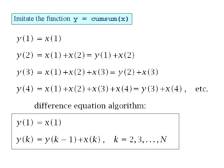
Imitate the function y = cumsum(x)

x = [10, -20, 30, 5, 25]; y(1) = x(1); for k=2: length(x) y(k) = y(k-1) + x(k); end for-loop >> y y = 10 -10 20 70 75 100 >> y = cumsum(x) y = 10 -10 20

x = [10, -20, 30, 5, 25]; y(1) = x(1); k = 2; while k <= length(x) y(k) = y(k-1) + x(k); k = k+1; end conventional while-loop, it computes the values, y(2), k=3; y(3), k=4; etc. y(1) = x(1); k = 2; while 1 if k > length(x), break; end y(k) = y(k-1) + x(k); k = k+1; end forever while-loop

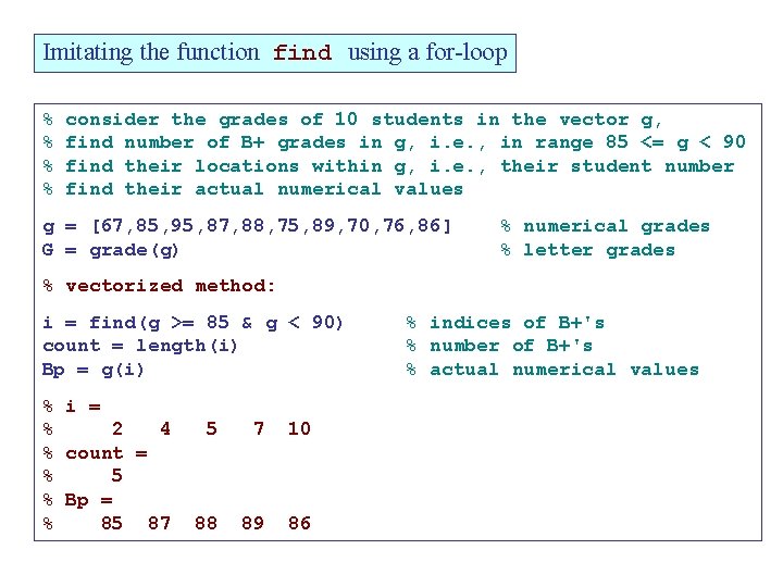
Imitating the function find using a for-loop % % consider the grades of 10 students in the vector g, find number of B+ grades in g, i. e. , in range 85 <= g < 90 find their locations within g, i. e. , their student number find their actual numerical values g = [67, 85, 95, 87, 88, 75, 89, 70, 76, 86] G = grade(g) % numerical grades % letter grades % vectorized method: i = find(g >= 85 & g < 90) count = length(i) Bp = g(i) % i = % 2 4 % count = % 5 % Bp = % 85 87 5 7 10 88 89 86 % indices of B+'s % number of B+'s % actual numerical values

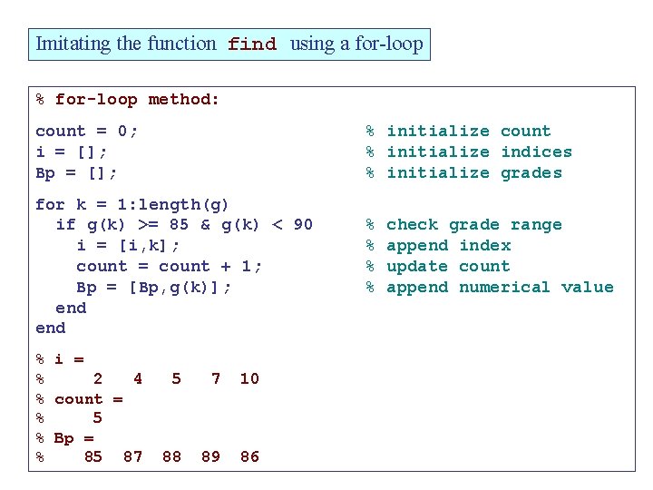
Imitating the function find using a for-loop % for-loop method: count = 0; i = []; Bp = []; % initialize count % initialize indices % initialize grades for k = 1: length(g) if g(k) >= 85 & g(k) < 90 i = [i, k]; count = count + 1; Bp = [Bp, g(k)]; end % i = % 2 4 % count = % 5 % Bp = % 85 87 5 7 10 88 89 86 % % check grade range append index update count append numerical value

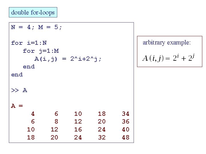
double for-loops N = 4; M = 5; arbitrary example: for i=1: N for j=1: M A(i, j) = 2^i+2^j; end >> A A = 4 6 10 18 6 8 12 20 10 12 16 24 18 20 24 32 34 36 40 48

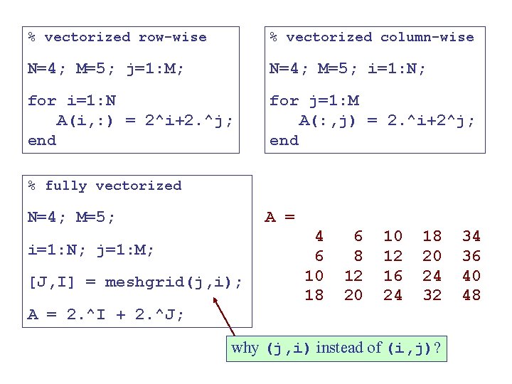
% vectorized row-wise % vectorized column-wise N=4; M=5; j=1: M; N=4; M=5; i=1: N; for i=1: N A(i, : ) = 2^i+2. ^j; end for j=1: M A(: , j) = 2. ^i+2^j; end % fully vectorized A = N=4; M=5; i=1: N; j=1: M; [J, I] = meshgrid(j, i); 4 6 10 18 6 8 12 20 10 12 16 24 18 20 24 32 A = 2. ^I + 2. ^J; why (j, i) instead of (i, j)? 34 36 40 48

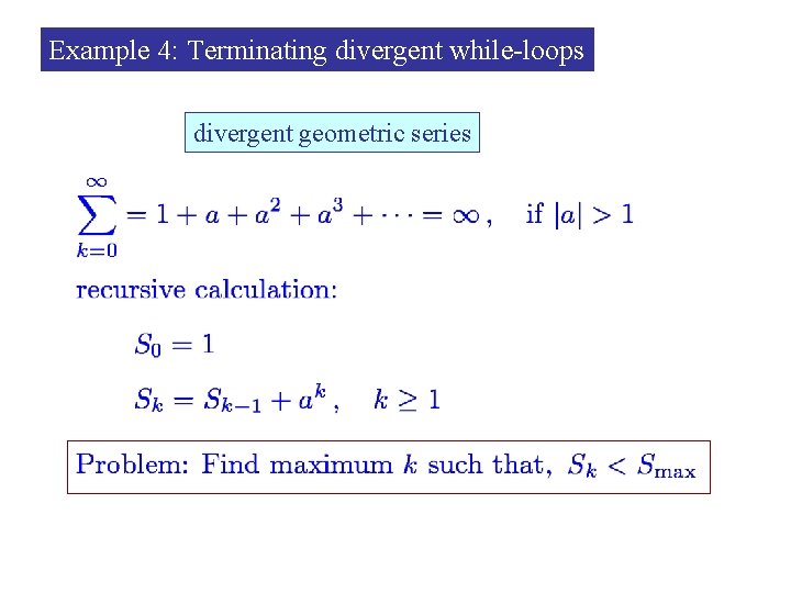
Example 4: Terminating divergent while-loops divergent geometric series

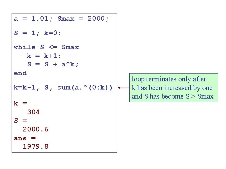
a = 1. 01; Smax = 2000; S = 1; k=0; while S <= Smax k = k+1; S = S + a^k; end k=k-1, S, sum(a. ^(0: k)) k = 304 S = 2000. 6 ans = 1979. 8 loop terminates only after k has been increased by one and S has become S > Smax

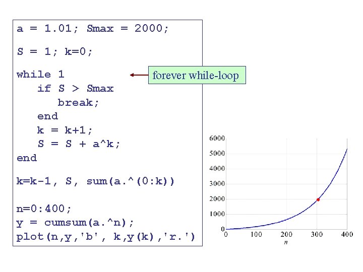
a = 1. 01; Smax = 2000; S = 1; k=0; while 1 if S > Smax break; end k = k+1; S = S + a^k; end forever while-loop k=k-1, S, sum(a. ^(0: k)) n=0: 400; y = cumsum(a. ^n); plot(n, y, 'b', k, y(k), 'r. ')

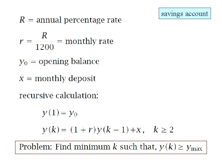
savings account

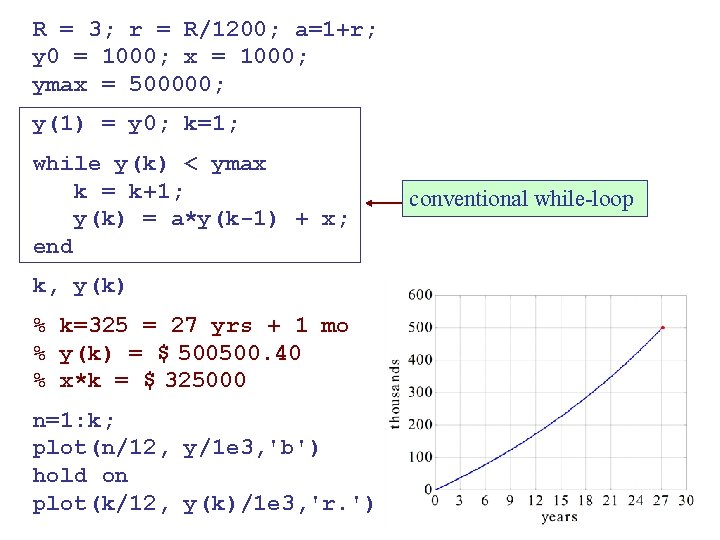
R = 3; r = R/1200; a=1+r; y 0 = 1000; x = 1000; ymax = 500000; y(1) = y 0; k=1; while y(k) < ymax k = k+1; y(k) = a*y(k-1) + x; end k, y(k) % k=325 = 27 yrs + 1 mo % y(k) = $ 500500. 40 % x*k = $ 325000 n=1: k; plot(n/12, y/1 e 3, 'b') hold on plot(k/12, y(k)/1 e 3, 'r. ') conventional while-loop

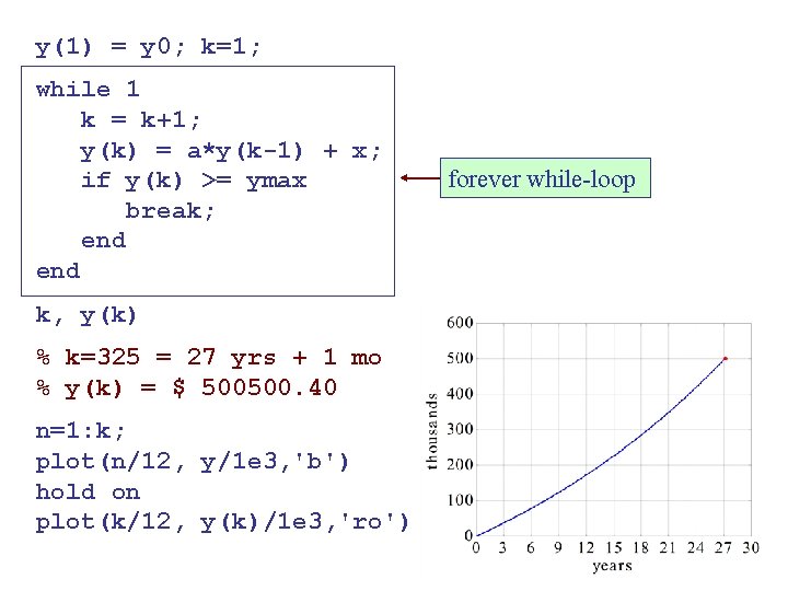
y(1) = y 0; k=1; while 1 k = k+1; y(k) = a*y(k-1) + x; if y(k) >= ymax break; end k, y(k) % k=325 = 27 yrs + 1 mo % y(k) = $ 500500. 40 n=1: k; plot(n/12, y/1 e 3, 'b') hold on plot(k/12, y(k)/1 e 3, 'ro') forever while-loop

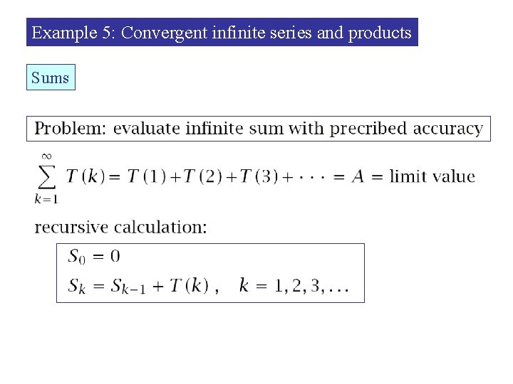
Example 5: Convergent infinite series and products Sums

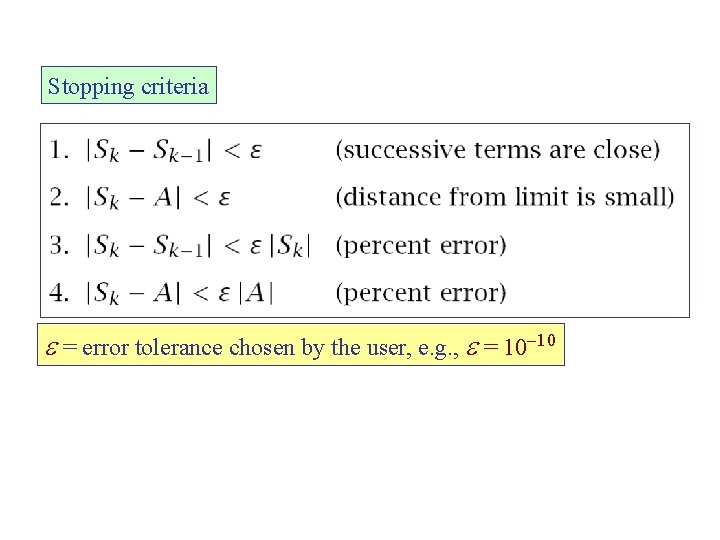
Stopping criteria e = error tolerance chosen by the user, e. g. , e = 10 -10

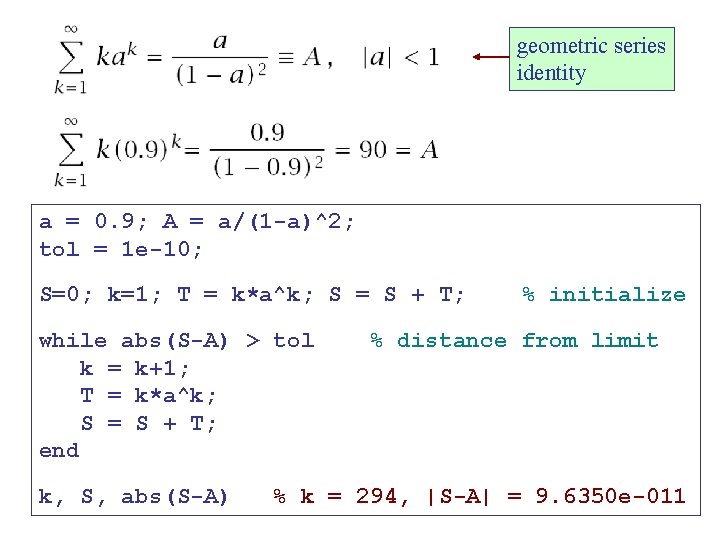
geometric series identity a = 0. 9; A = a/(1 -a)^2; tol = 1 e-10; S=0; k=1; T = k*a^k; S = S + T; while abs(S-A) > tol k = k+1; T = k*a^k; S = S + T; end k, S, abs(S-A) % initialize % distance from limit % k = 294, |S-A| = 9. 6350 e-011

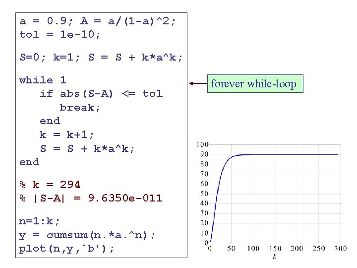
a = 0. 9; A = a/(1 -a)^2; tol = 1 e-10; S=0; k=1; S = S + k*a^k; while 1 if abs(S-A) <= tol break; end k = k+1; S = S + k*a^k; end % k = 294 % |S-A| = 9. 6350 e-011 n=1: k; y = cumsum(n. *a. ^n); plot(n, y, 'b'); forever while-loop

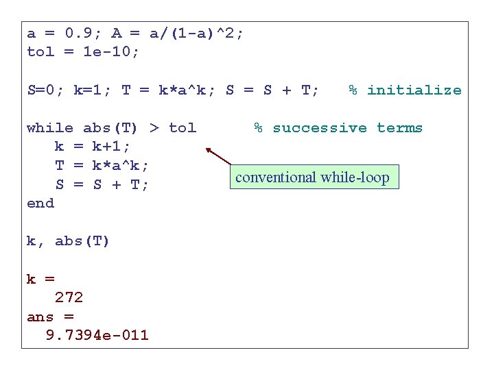
a = 0. 9; A = a/(1 -a)^2; tol = 1 e-10; S=0; k=1; T = k*a^k; S = S + T; while abs(T) > tol k = k+1; T = k*a^k; S = S + T; end k, abs(T) k = 272 ans = 9. 7394 e-011 % initialize % successive terms conventional while-loop

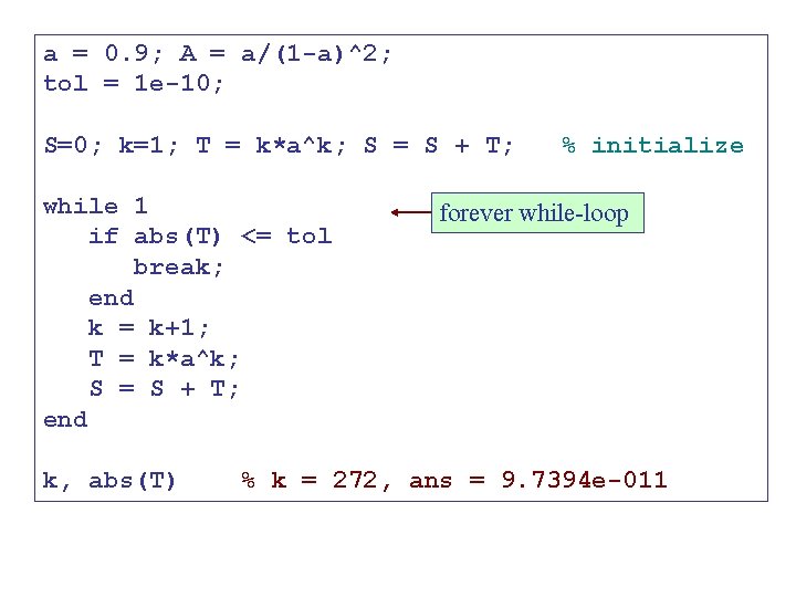
a = 0. 9; A = a/(1 -a)^2; tol = 1 e-10; S=0; k=1; T = k*a^k; S = S + T; while 1 if abs(T) <= tol break; end k = k+1; T = k*a^k; S = S + T; end k, abs(T) % initialize forever while-loop % k = 272, ans = 9. 7394 e-011

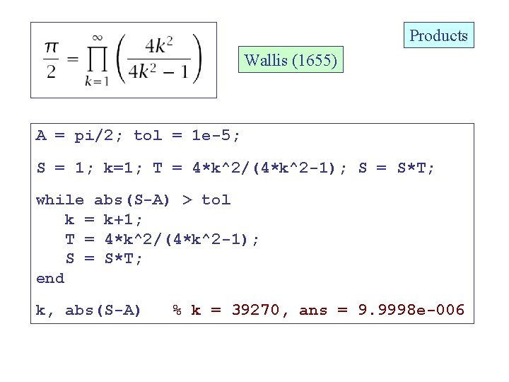
Products Wallis (1655) A = pi/2; tol = 1 e-5; S = 1; k=1; T = 4*k^2/(4*k^2 -1); S = S*T; while abs(S-A) > tol k = k+1; T = 4*k^2/(4*k^2 -1); S = S*T; end k, abs(S-A) % k = 39270, ans = 9. 9998 e-006

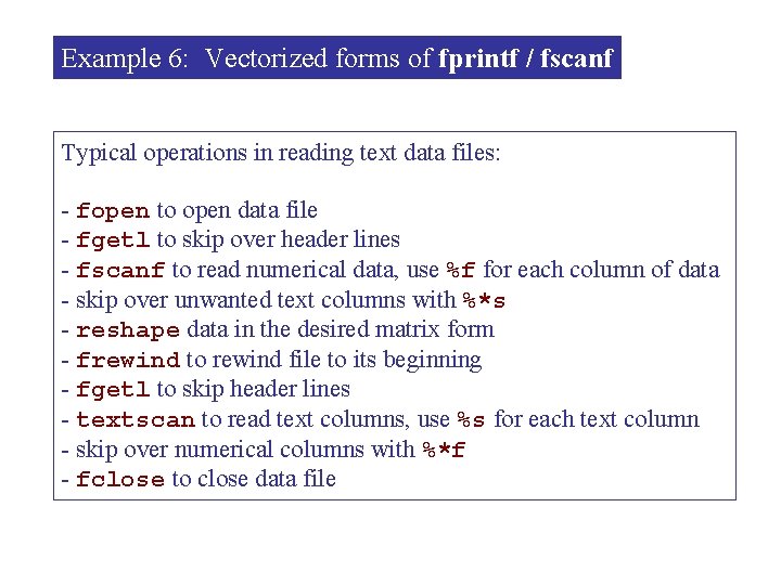
Example 6: Vectorized forms of fprintf / fscanf Typical operations in reading text data files: - fopen to open data file - fgetl to skip over header lines - fscanf to read numerical data, use %f for each column of data - skip over unwanted text columns with %*s - reshape data in the desired matrix form - frewind to rewind file to its beginning - fgetl to skip header lines - textscan to read text columns, use %s for each text column - skip over numerical columns with %*f - fclose to close data file

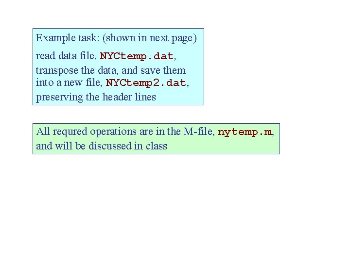
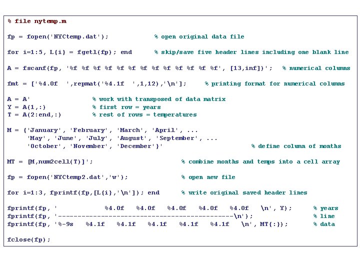
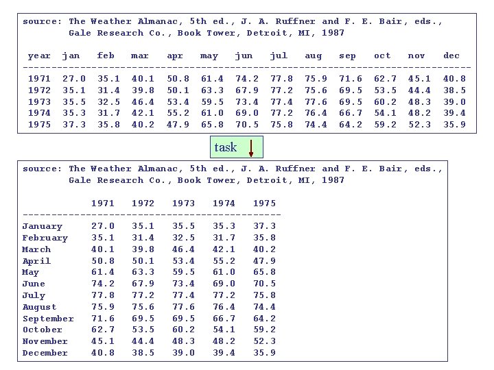
Example task: (shown in next page) read data file, NYCtemp. dat, transpose the data, and save them into a new file, NYCtemp 2. dat, preserving the header lines All requred operations are in the M-file, nytemp. m, and will be discussed in class

% file nytemp. m fp = fopen('NYCtemp. dat'); % open original data file for i=1: 5, L{i} = fgetl(fp); end % skip/save five header lines including one blank line A = fscanf(fp, '%f %f %f %f', [13, inf])'; fmt = ['%4. 0 f A = A' Y = A(1, : ) T = A(2: end, : ) ', repmat('%4. 1 f ', 1, 12), 'n']; % numerical columns % printing format for numerical columns % work with transposed of data matrix % first row = years % rest of rows = temperatures M = {'January', 'February', 'March', 'April', . . . 'May', 'June', 'July', 'August', 'September', . . . 'October', 'November', 'December'}' % define column of months MT = [M, num 2 cell(T)]'; % combine months and temps into a cell array fp = fopen('NYCtemp 2. dat', 'w'); % open new file for i=1: 3, fprintf(fp, [L{i}, 'n']); end % write original saved header lines fprintf(fp, ' %4. 0 f n', Y); fprintf(fp, '-----------------------n'); fprintf(fp, '%-9 s %4. 1 f n', MT{: }); fclose(fp); % years % line % data

source: The Weather Almanac, 5 th ed. , J. A. Ruffner and F. E. Bair, eds. , Gale Research Co. , Book Tower, Detroit, MI, 1987 year jan feb mar apr may jun jul aug sep oct nov dec ---------------------------------------1971 27. 0 35. 1 40. 1 50. 8 61. 4 74. 2 77. 8 75. 9 71. 6 62. 7 45. 1 40. 8 1972 35. 1 31. 4 39. 8 50. 1 63. 3 67. 9 77. 2 75. 6 69. 5 53. 5 44. 4 38. 5 1973 35. 5 32. 5 46. 4 53. 4 59. 5 73. 4 77. 6 69. 5 60. 2 48. 3 39. 0 1974 35. 3 31. 7 42. 1 55. 2 61. 0 69. 0 77. 2 76. 4 66. 7 54. 1 48. 2 39. 4 1975 37. 3 35. 8 40. 2 47. 9 65. 8 70. 5 75. 8 74. 4 64. 2 59. 2 52. 3 35. 9 task source: The Weather Almanac, 5 th ed. , J. A. Ruffner and F. E. Bair, eds. , Gale Research Co. , Book Tower, Detroit, MI, 1987 1971 1972 1973 1974 1975 ----------------------January 27. 0 35. 1 35. 5 35. 3 37. 3 February 35. 1 31. 4 32. 5 31. 7 35. 8 March 40. 1 39. 8 46. 4 42. 1 40. 2 April 50. 8 50. 1 53. 4 55. 2 47. 9 May 61. 4 63. 3 59. 5 61. 0 65. 8 June 74. 2 67. 9 73. 4 69. 0 70. 5 July 77. 8 77. 2 77. 4 77. 2 75. 8 August 75. 9 75. 6 77. 6 76. 4 74. 4 September 71. 6 69. 5 66. 7 64. 2 October 62. 7 53. 5 60. 2 54. 1 59. 2 November 45. 1 44. 4 48. 3 48. 2 52. 3 December 40. 8 38. 5 39. 0 39. 4 35. 9