Routing Algorithms 14 740 Fundamentals of Computer Networks

Routing Algorithms 14 -740: Fundamentals of Computer Networks Bcredit: ill Nace Material from Computer Networking: A Top Down Approach, 6 th edition. J. F. Kurose and K. W. Ross

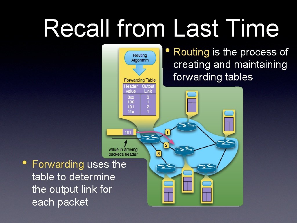
Recall from Last Time • Routing is the process of creating and maintaining forwarding tables • Forwarding uses the table to determine the output link for each packet

traceroute • Routing Theory: Graphs and Overview • Link State Algorithms • Distance Vector Algorithms 14 -740: Spring 2018 3

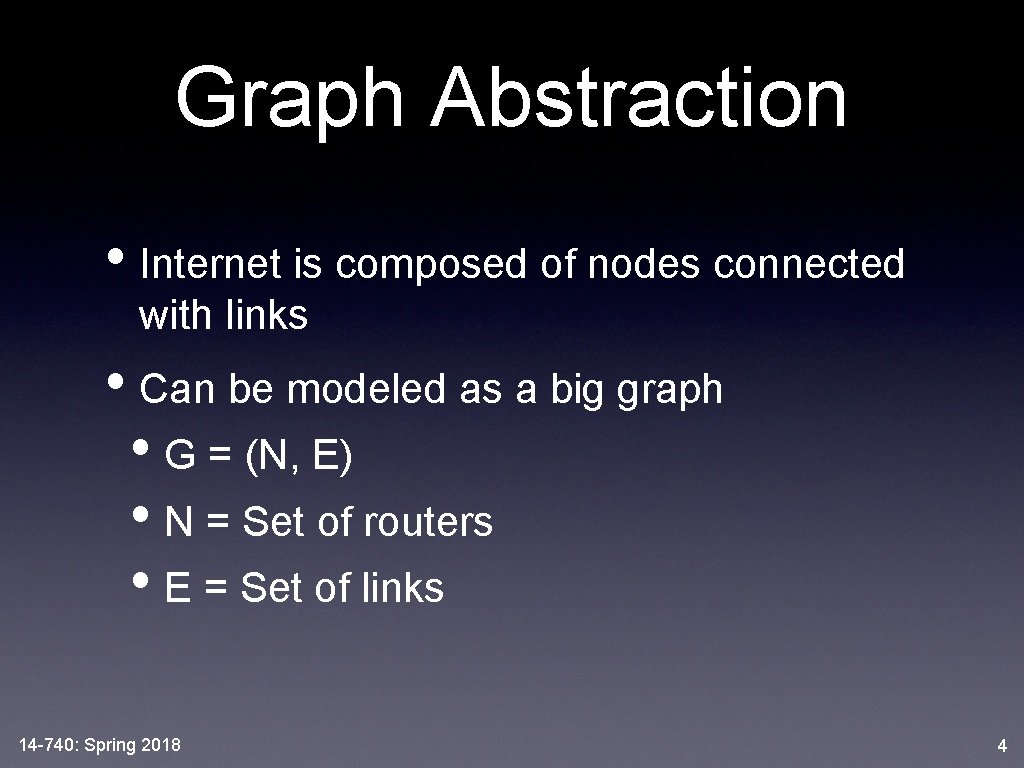
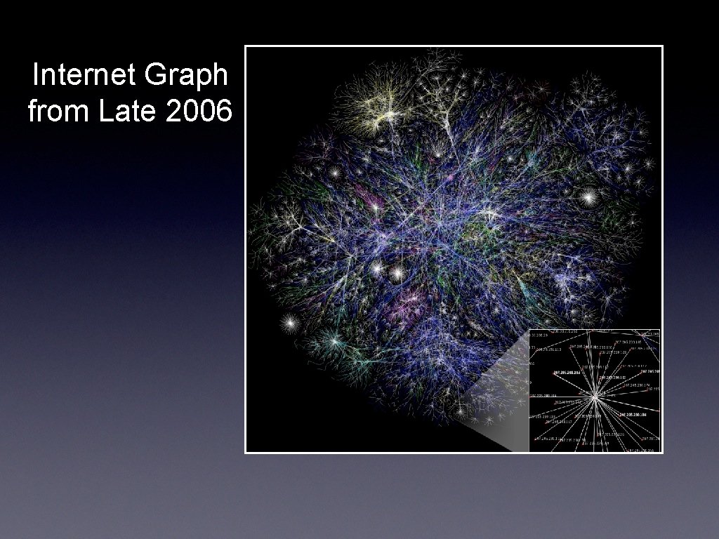
Graph Abstraction • Internet is composed of nodes connected with links • Can be modeled as a big graph • G = (N, E) • N = Set of routers • E = Set of links 14 -740: Spring 2018 4

Internet Graph from Late 2006

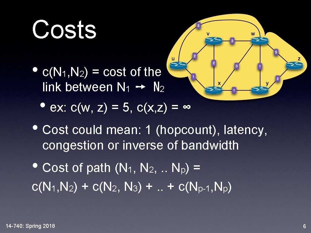
Costs • c(N 1, N 2) = cost of the link between N 1 ➙ N 2 • ex: c(w, z) = 5, c(x, z) = ∞ • Cost could mean: 1 (hopcount), latency, congestion or inverse of bandwidth • Cost of path (N 1, N 2, . . Np) = c(N 1, N 2) + c(N 2, N 3) +. . + c(Np-1, Np) 14 -740: Spring 2018 6

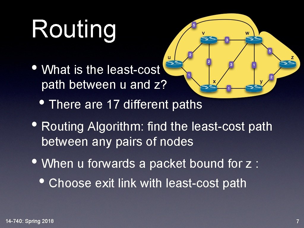
Routing • What is the least-cost path between u and z? • There are 17 different paths • Routing Algorithm: find the least-cost path between any pairs of nodes • When u forwards a packet bound for z : • Choose exit link with least-cost path 14 -740: Spring 2018 7

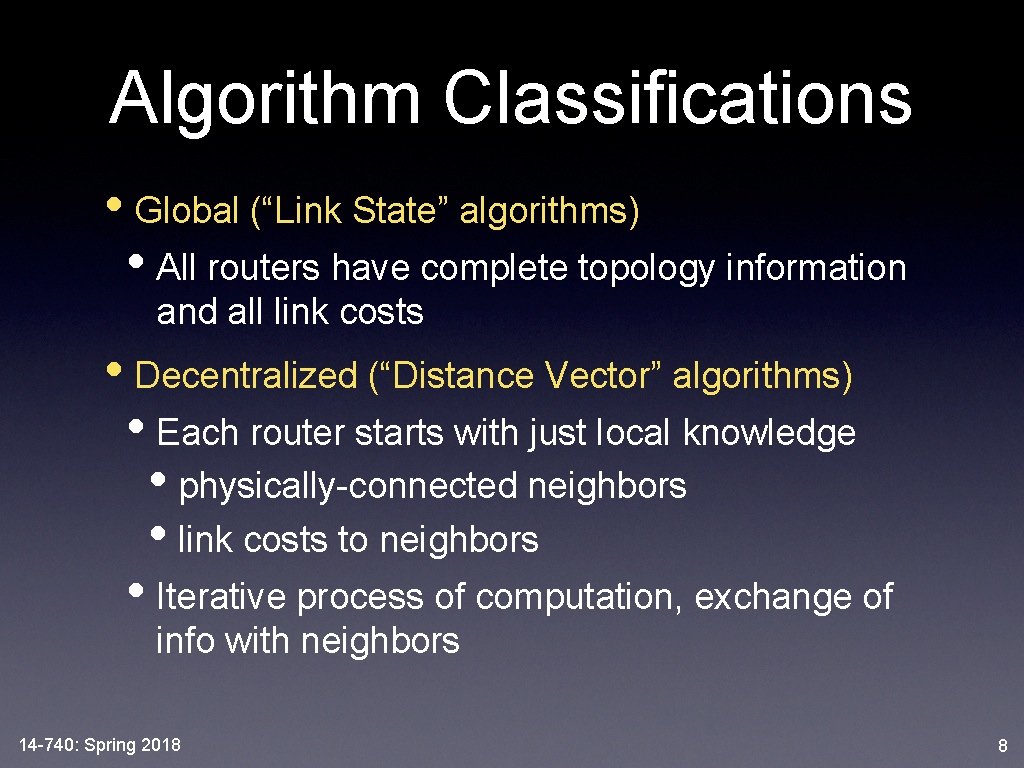
Algorithm Classifications • Global (“Link State” algorithms) • All routers have complete topology information and all link costs • Decentralized (“Distance Vector” algorithms) • Each router starts with just local knowledge • physically-connected neighbors • link costs to neighbors • Iterative process of computation, exchange of info with neighbors 14 -740: Spring 2018 8

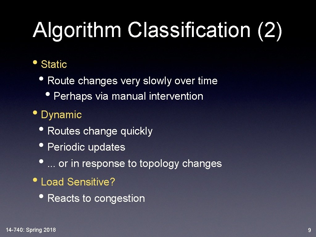
Algorithm Classification (2) • Static • Route changes very slowly over time • Perhaps via manual intervention • Dynamic • Routes change quickly • Periodic updates • . . . or in response to topology changes • Load Sensitive? • Reacts to congestion 14 -740: Spring 2018 9

traceroute • Routing Theory: Graphs and Overview • Link State Algorithms • Distance Vector Algorithms 14 -740: Spring 2018 10

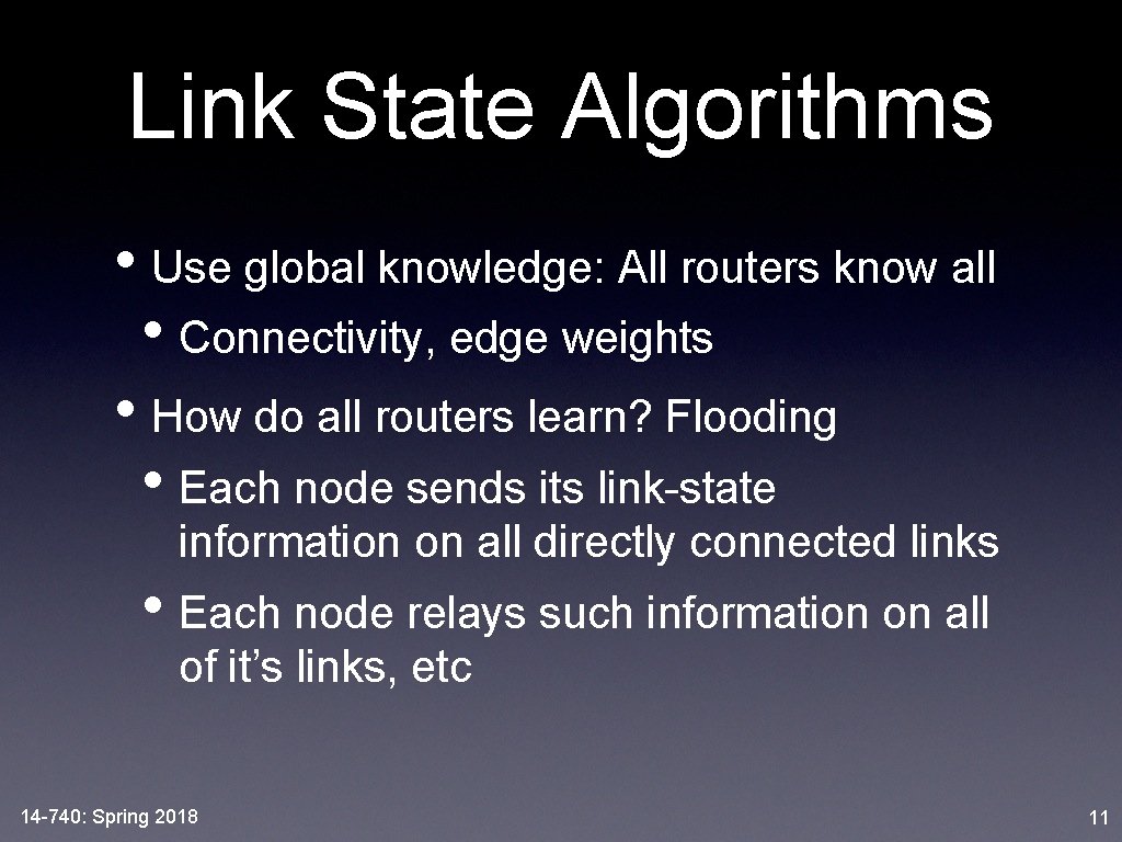
Link State Algorithms • Use global knowledge: All routers know all • Connectivity, edge weights • How do all routers learn? Flooding • Each node sends its link-state information on all directly connected links • Each node relays such information on all of it’s links, etc 14 -740: Spring 2018 11

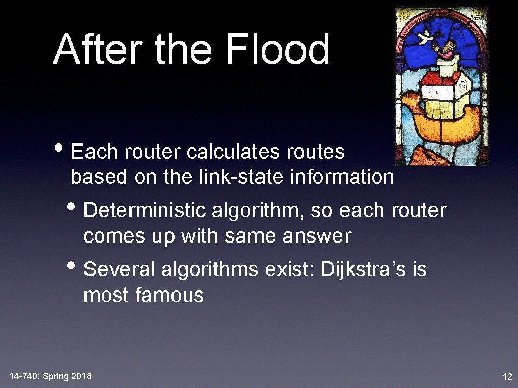
After the Flood • Each router calculates routes based on the link-state information • Deterministic algorithm, so each router comes up with same answer • Several algorithms exist: Dijkstra’s is most famous 14 -740: Spring 2018 12

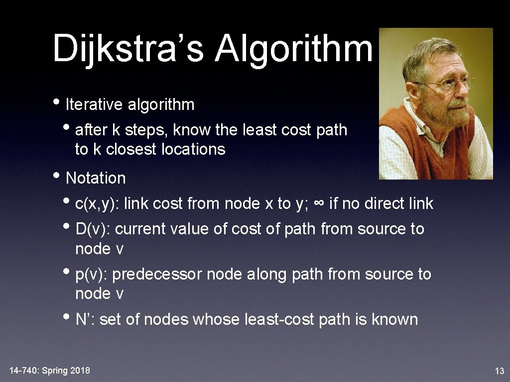
Dijkstra’s Algorithm • Iterative algorithm • after k steps, know the least cost path to k closest locations • Notation • c(x, y): link cost from node x to y; ∞ if no direct link • D(v): current value of cost of path from source to node v • p(v): predecessor node along path from source to node v • N’: set of nodes whose least-cost path is known 14 -740: Spring 2018 13

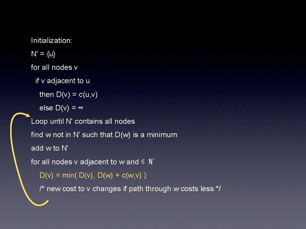
Initialization: N' = {u} for all nodes v if v adjacent to u then D(v) = c(u, v) else D(v) = ∞ Loop until N' contains all nodes find w not in N' such that D(w) is a minimum add w to N' for all nodes v adjacent to w and ∉ N' D(v) = min( D(v), D(w) + c(w, v) ) /* new cost to v changes if path through w costs less */

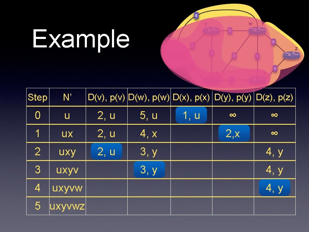
Example Step N’ 0 u 2, u 5, u 1 ux 2, u 4, x 2 uxy 2, u 3, y 4, y 3 uxyv 3, y 4 uxyvw 5 uxyvwz D(v), p(v) D(w), p(w) D(x), p(x) D(y), p(y) D(z), p(z) 1, u ∞ ∞ 2, x ∞ 4, y

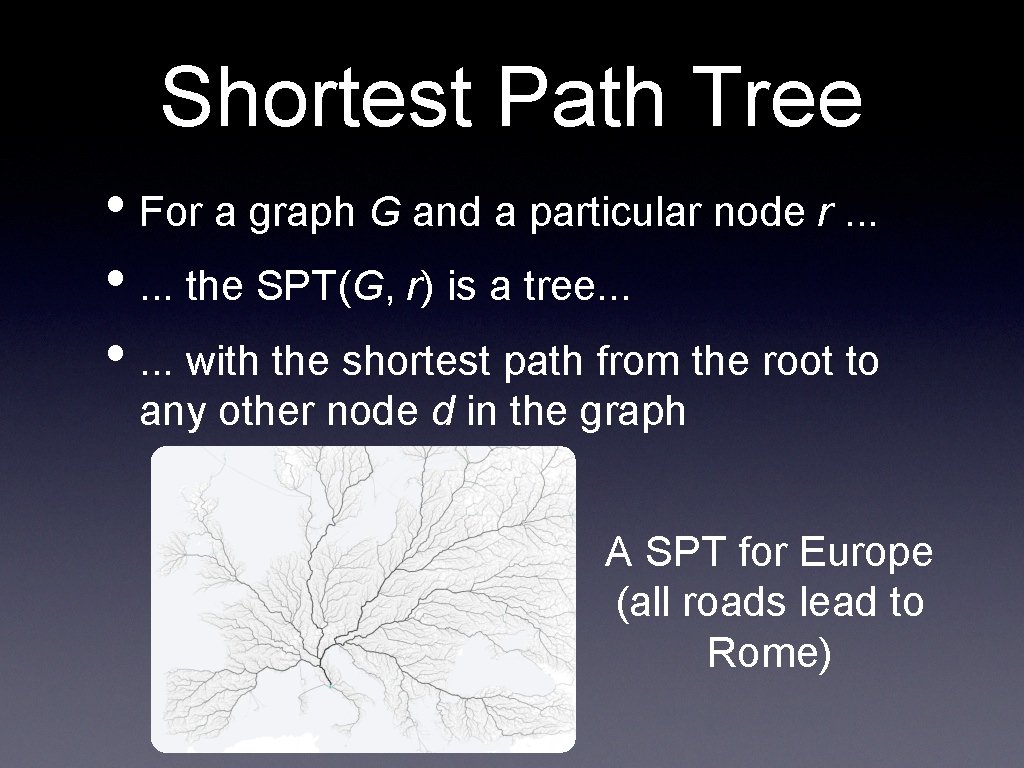
Shortest Path Tree • For a graph G and a particular node r. . . • . . . the SPT(G, r) is a tree. . . • . . . with the shortest path from the root to any other node d in the graph A SPT for Europe (all roads lead to Rome)

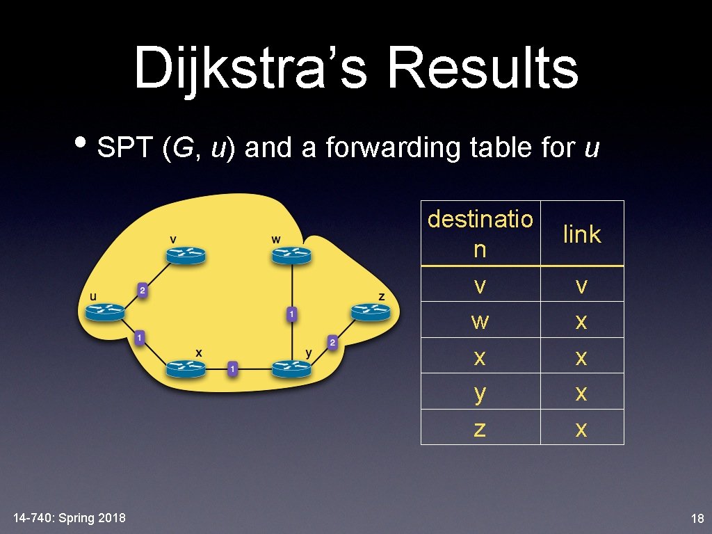
Dijkstra’s Results • SPT (G, u) and a forwarding table for u destinatio n v w x y z 14 -740: Spring 2018 link v x x 18

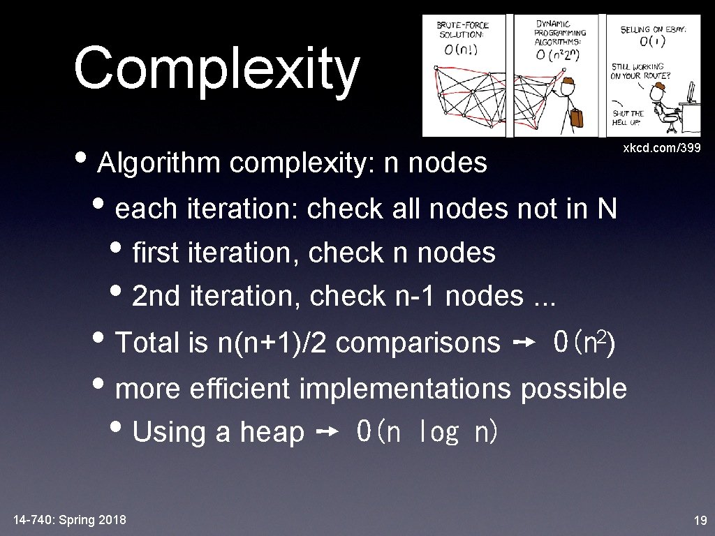
Complexity • Algorithm complexity: n nodes • each iteration: check all nodes not in N • first iteration, check n nodes • 2 nd iteration, check n-1 nodes. . . 2 • Total is n(n+1)/2 comparisons ➙ O(n ) • more efficient implementations possible • Using a heap ➙ O(n log n) xkcd. com/399 14 -740: Spring 2018 19

traceroute • Routing Theory: Graphs and Overview • Link State Algorithms • Distance Vector Algorithms 14 -740: Spring 2018 20

Distance-Vector Algs • Still need to distribute local information • Message exchange rather than flooding • Each node exchanges distance vector with neighboring nodes • 1 d map of nodes to distances 14 -740: Spring 2018 21

Routing Algorithm • Iterative: Each local iteration caused by. . • . . . A change in local link cost • . . . or DV update message from neighbor • Distributed • Each node autonomously computes based on local knowledge. . . • . . . which, after “enough” iterations is communicated to the world 14 -740: Spring 2018 22

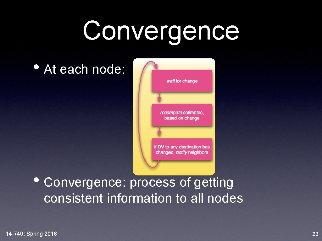
Convergence • At each node: • Convergence: process of getting consistent information to all nodes 14 -740: Spring 2018 23

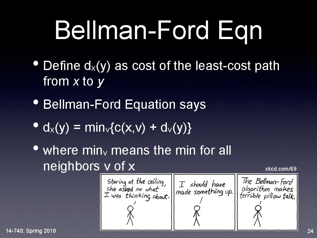
Bellman-Ford Eqn • Define dx(y) as cost of the least-cost path from x to y • Bellman-Ford Equation says • dx(y) = minv{c(x, v) + dv(y)} • where minv means the min for all neighbors v of x 14 -740: Spring 2018 xkcd. com/69 24

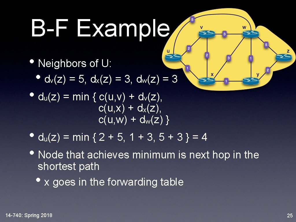
B-F Example • Neighbors of U: • dv(z) = 5, dx(z) = 3, dw(z) = 3 • du(z) = min { c(u, v) + dv(z), c(u, x) + dx(z), c(u, w) + dw(z) } • du(z) = min { 2 + 5, 1 + 3, 5 + 3 } = 4 • Node that achieves minimum is next hop in the shortest path • x goes in the forwarding table 14 -740: Spring 2018 25

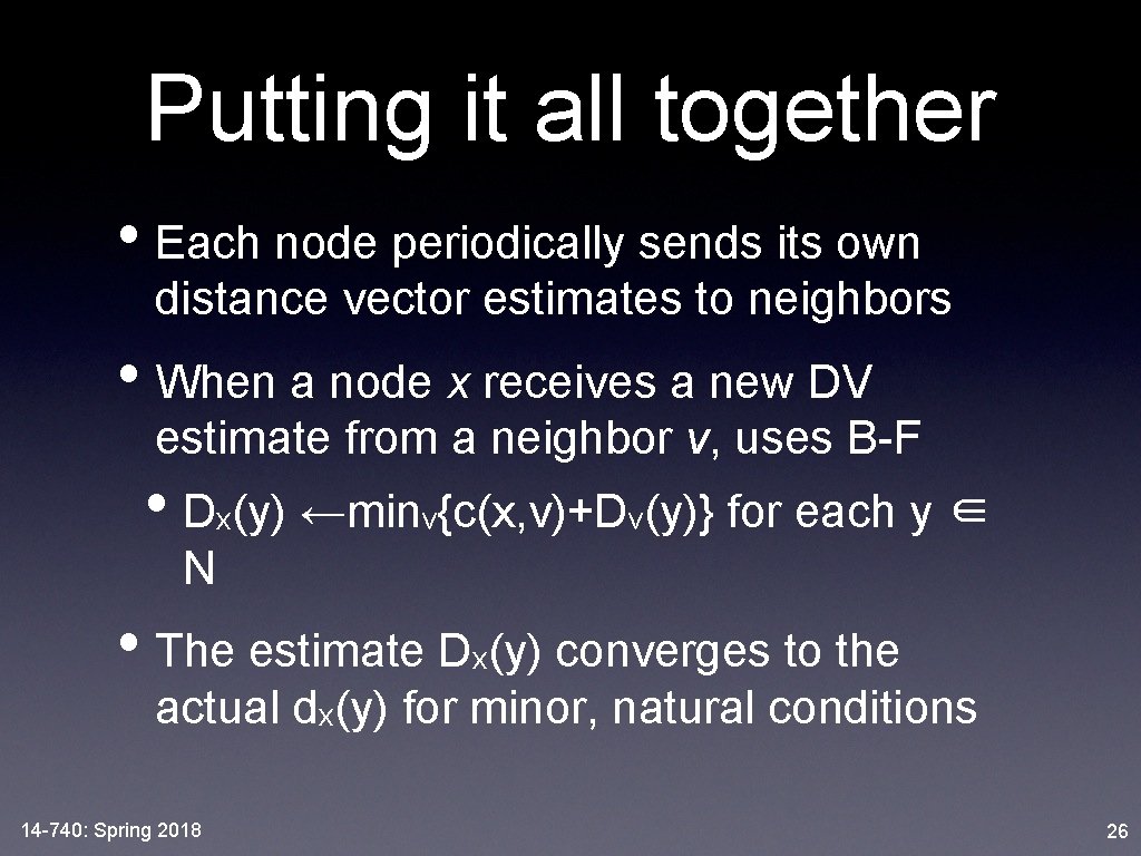
Putting it all together • Each node periodically sends its own distance vector estimates to neighbors • When a node x receives a new DV estimate from a neighbor v, uses B-F • Dx(y) ←minv{c(x, v)+Dv(y)} for each y ∈ N • The estimate Dx(y) converges to the actual dx(y) for minor, natural conditions 14 -740: Spring 2018 26

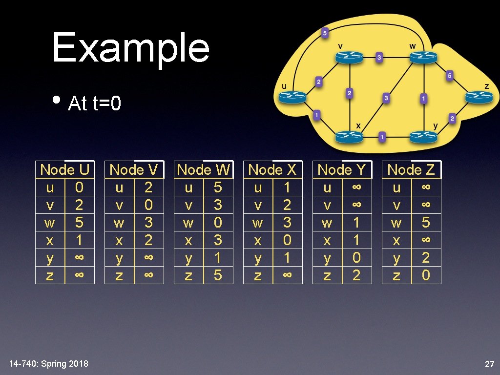
Example • At t=0 Node U u 0 v 2 w 5 x 1 y ∞ z ∞ 14 -740: Spring 2018 Node V u 2 v 0 w 3 x 2 y ∞ z ∞ Node W u 5 v 3 w 0 x 3 y 1 z 5 Node X u 1 v 2 w 3 x 0 y 1 z ∞ Node Y u ∞ v ∞ w 1 x 1 y 0 z 2 Node Z u ∞ v ∞ w 5 x ∞ y 2 z 0 27

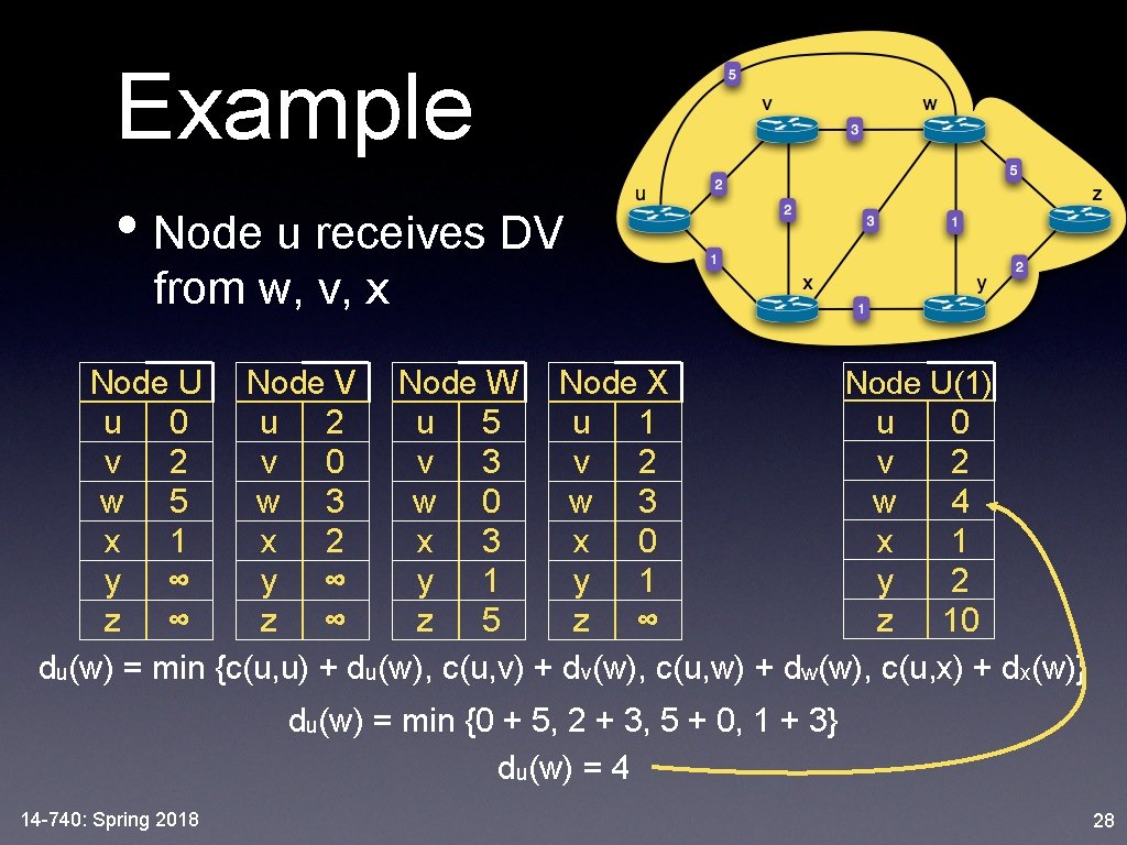
Example • Node u receives DV from w, v, x Node U(1) Node U Node V Node W Node X u 0 u 2 u 5 u 1 v 2 v 0 v 3 v 2 w 4 w 5 w 3 w 0 w 3 x 1 x 2 x 3 x 0 y 2 y ∞ y 1 z 10 z ∞ z 5 z ∞ du(w) = min {c(u, u) + du(w), c(u, v) + dv(w), c(u, w) + dw(w), c(u, x) + dx(w)} du(w) = min {0 + 5, 2 + 3, 5 + 0, 1 + 3} du(w) = 4 14 -740: Spring 2018 28

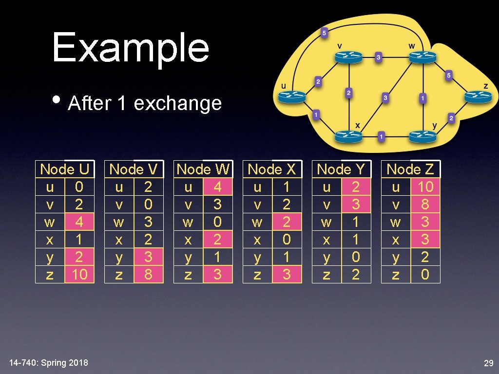
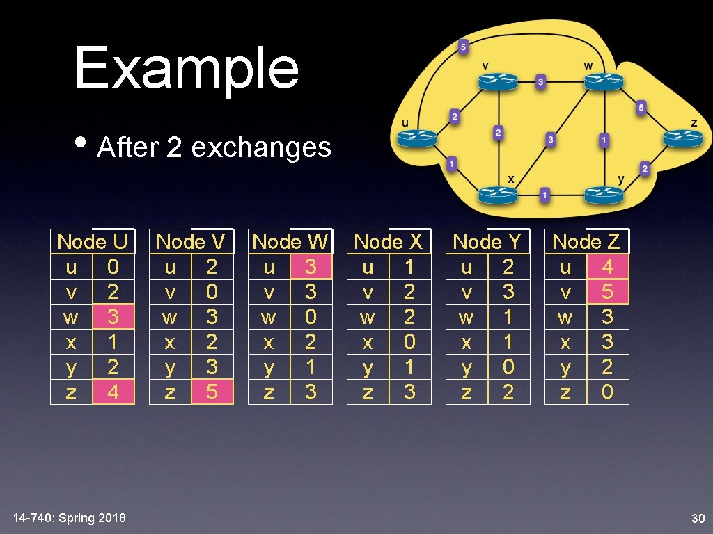
Example • After 1 exchange Node U u 0 v 2 w 4 x 1 y 2 z 10 14 -740: Spring 2018 Node V u 2 v 0 w 3 x 2 y 3 z 8 Node W u 4 v 3 w 0 x 2 y 1 z 3 Node X u 1 v 2 w 2 x 0 y 1 z 3 Node Y u 2 v 3 w 1 x 1 y 0 z 2 Node Z u 10 v 8 w 3 x 3 y 2 z 0 29

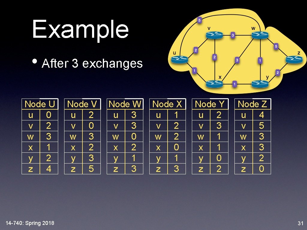
Example • After 2 exchanges Node U u 0 v 2 w 3 x 1 y 2 z 4 14 -740: Spring 2018 Node V u 2 v 0 w 3 x 2 y 3 z 5 Node W u 3 v 3 w 0 x 2 y 1 z 3 Node X u 1 v 2 w 2 x 0 y 1 z 3 Node Y u 2 v 3 w 1 x 1 y 0 z 2 Node Z u 4 v 5 w 3 x 3 y 2 z 0 30

Example • After 3 exchanges Node U u 0 v 2 w 3 x 1 y 2 z 4 14 -740: Spring 2018 Node V u 2 v 0 w 3 x 2 y 3 z 5 Node W u 3 v 3 w 0 x 2 y 1 z 3 Node X u 1 v 2 w 2 x 0 y 1 z 3 Node Y u 2 v 3 w 1 x 1 y 0 z 2 Node Z u 4 v 5 w 3 x 3 y 2 z 0 31

Dynamics • If a link cost changes • Node detects local link cost change, updates own forwarding table (recalculates DV) • If DV changes, will notify neighbors • “Good News travels fast” (one link-radius per exchange) 14 -740: Spring 2018 32

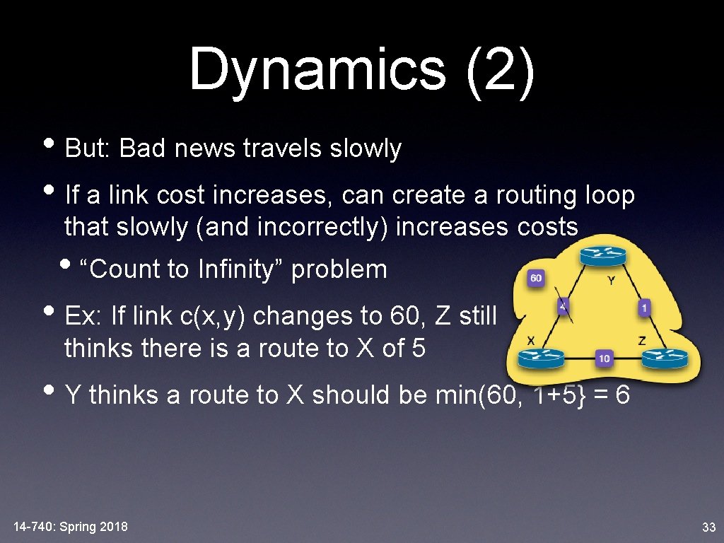
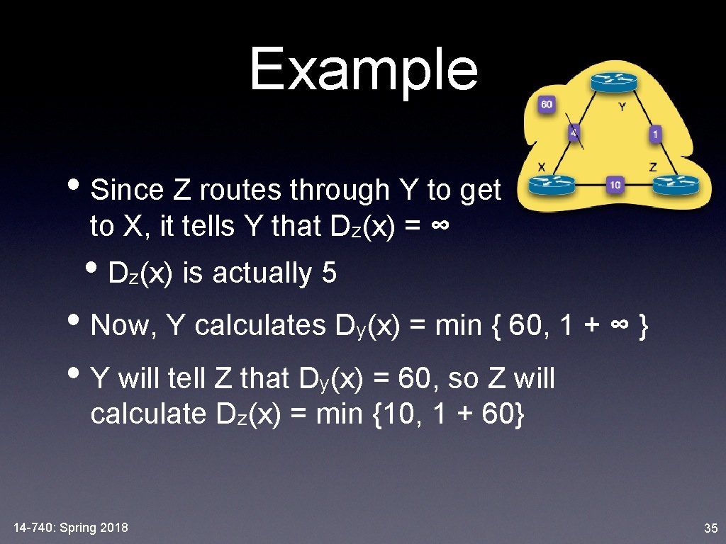
Dynamics (2) • But: Bad news travels slowly • If a link cost increases, can create a routing loop that slowly (and incorrectly) increases costs • “Count to Infinity” problem • Ex: If link c(x, y) changes to 60, Z still thinks there is a route to X of 5 • Y thinks a route to X should be min(60, 1+5} = 6 14 -740: Spring 2018 33

Stabilization Techniques • Split horizon • When a node sends a routing update to its neighbor, does not send those routes it learned from each neighbor back to that neighbor • Split horizon with poisoned reverse • Nodes advertise a cost of ∞ for a destination to the neighbor it routes through to that destination 14 -740: Spring 2018 34

Example • Since Z routes through Y to get to X, it tells Y that Dz(x) = ∞ • Dz(x) is actually 5 • Now, Y calculates Dy(x) = min { 60, 1 + ∞ } • Y will tell Z that Dy(x) = 60, so Z will calculate Dz(x) = min {10, 1 + 60} 14 -740: Spring 2018 35

Can also redefine ∞ • Assume maximum costs to get to anywhere is C • Do not let cost get > C in calculation • This bounds the time to “count to infinity” • Unfortunately, no technique completely solves the “count to infinity” problem • When routing loop contains 3+ nodes 14 -740: Spring 2018 36

Comparison • Message Complexity • LS: with n nodes, E links, O(n. E) messages sent • DV: exchange between neighbors only • Speed of Convergence • LS: After correct message exchange • DV: Varies. May be routing loops 14 -740: Spring 2018 37

Comparison (2) • Robustness: what happens if router malfunctions? • LS: node can advertise incorrect link cost • each node computes only its own table • DV: node can advertise incorrect path cost • each node’s table used by others, error propagates thru network 14 -740: Spring 2018 38

Lesson Objectives • Now, you should be able to: • describe the differences between global / • decentralized and static / dynamic routing algorithms. Students should be able to describe different message complexity, convergence speeds, robustness and algorithm complexity calculate a forwarding table using Dijkstra's algorithm (which may include identifying and using proper variables and terms). Intermediate results may be required, such as an SPT or table of variable values 14 -740: Spring 2018 39

• You should be able to: • use Bellman-Ford equations to calculate a forwarding table for a DV routing algorithm. Intermediate values may be required, which may require knowing variable names and terms • describe how DV algorithms operate to pass updates • describe DV instability problems, such as “Count to Infinity” and the associated stabilization techniques • analyze DV instability examples