Queueing Theory 14 740 Fundamentals of Computer Networks

Queueing Theory 14 -740: Fundamentals of Computer Networks Credit: Bill Nace Material from Computer Networking: A Top Down Approach, 6 th edition. J. F. Kurose and K. W. Ross

traceroute • QT Overview • Performance Evaluation • Little’s Law • Rate Transition Diagrams • M/M/1 Systems • M/M/c Systems • Examples 14 -740: Fall 2017 2

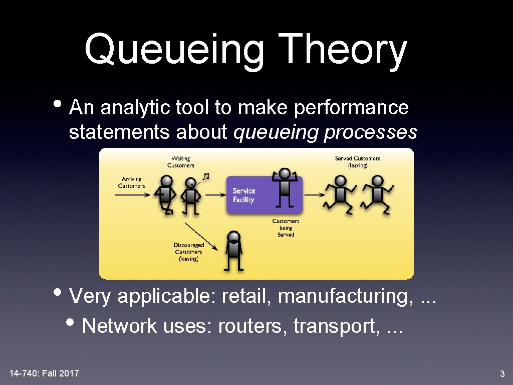
Queueing Theory • An analytic tool to make performance statements about queueing processes • Very applicable: retail, manufacturing, . . . • Network uses: routers, transport, . . . 14 -740: Fall 2017 3

Queueing System • Describe via six characteristics • Arrival pattern • Service pattern • Queue discipline • System capacity • # of service channels • # of service stages 14 -740: Fall 2017 4

#1: Arrival Pattern • Often, arrivals are stochastic • Need to know the PDF of interarrival times • Sometimes, arrive in batches or in bulk • Need the PDF of batch size • A stationary arrival pattern doesn’t change with time 14 -740: Fall 2017 5

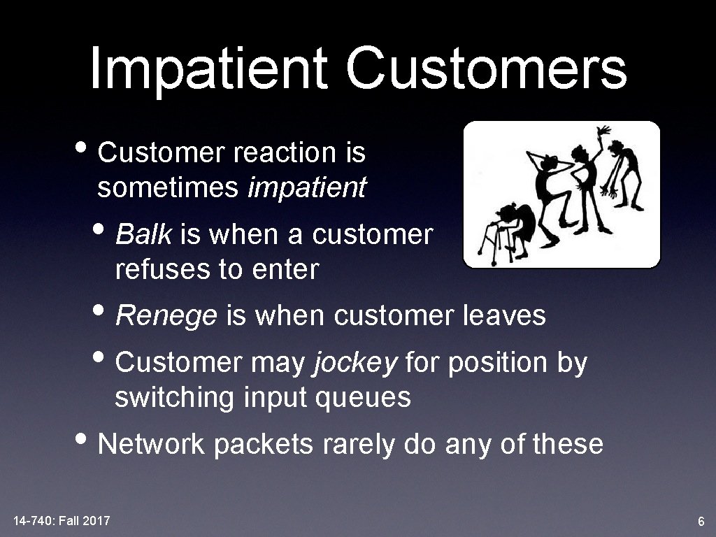
Impatient Customers • Customer reaction is sometimes impatient • Balk is when a customer refuses to enter • Renege is when customer leaves • Customer may jockey for position by switching input queues • Network packets rarely do any of these 14 -740: Fall 2017 6

#2: Service Pattern • Similar to arrival patterns, service patterns are often stochastic • Described by a PDF of customer service times • A state-dependent server changes based on the number of customers waiting • Server may get flustered or work faster • Service can be stationary or nonstationary 14 -740: Fall 2017 7

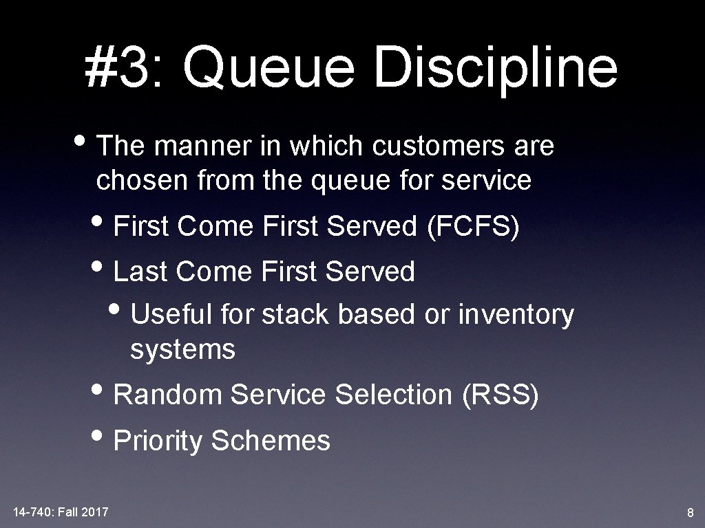
#3: Queue Discipline • The manner in which customers are chosen from the queue for service • First Come First Served (FCFS) • Last Come First Served • Useful for stack based or inventory systems • Random Service Selection (RSS) • Priority Schemes 14 -740: Fall 2017 8

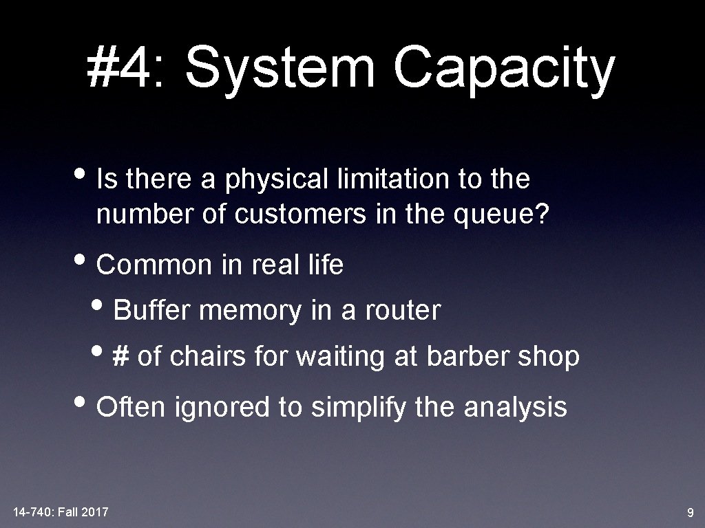
#4: System Capacity • Is there a physical limitation to the number of customers in the queue? • Common in real life • Buffer memory in a router • # of chairs for waiting at barber shop • Often ignored to simplify the analysis 14 -740: Fall 2017 9

#5: Multiple Service Channels • Adding servers increases capacity • How do customers wait? • Single queue can feed many servers • Each server may have its own queue 14 -740: Fall 2017 10

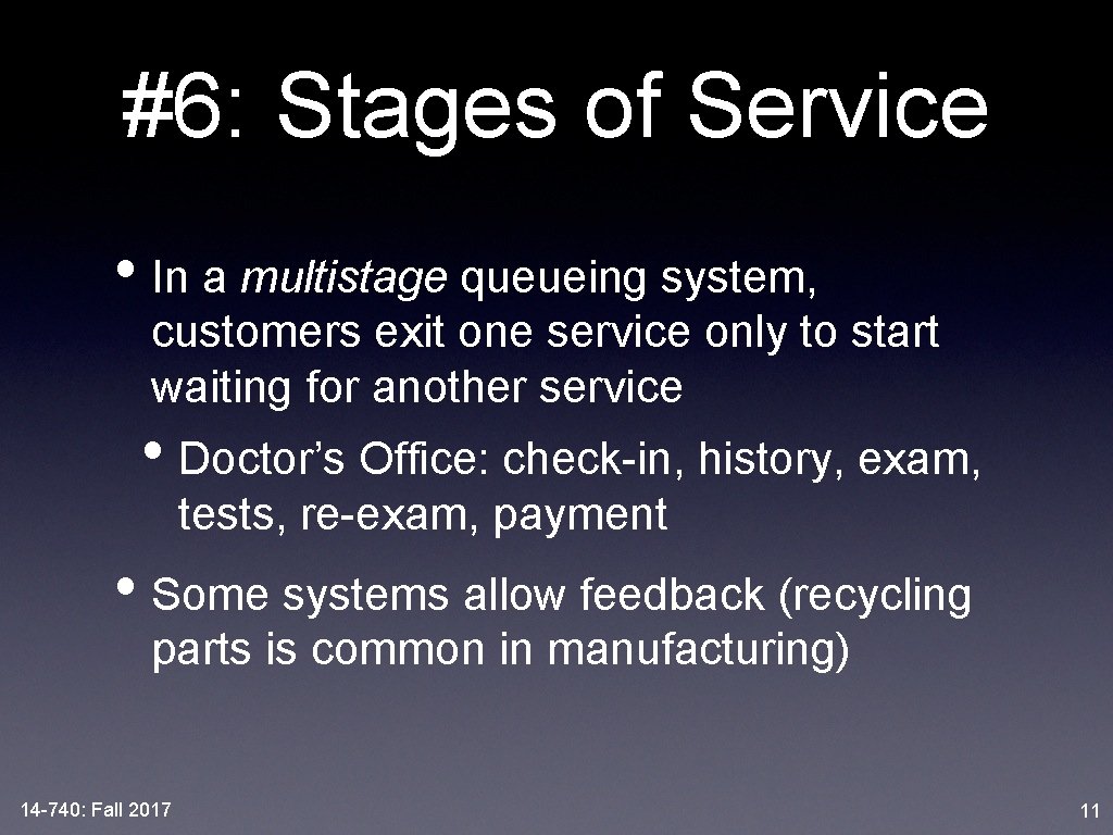
#6: Stages of Service • In a multistage queueing system, customers exit one service only to start waiting for another service • Doctor’s Office: check-in, history, exam, tests, re-exam, payment • Some systems allow feedback (recycling parts is common in manufacturing) 14 -740: Fall 2017 11

Greek • 14 -740: Fall 2017

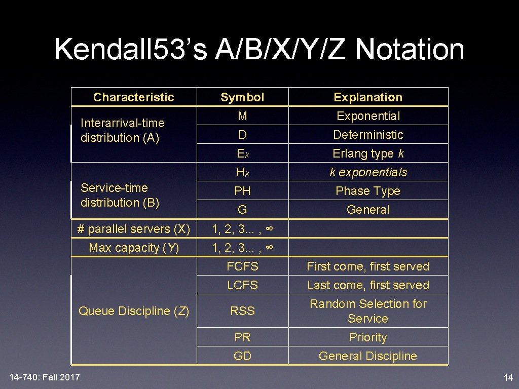
Kendall 53’s A/B/X/Y/Z Notation Characteristic Interarrival-time distribution (A) Service-time distribution (B) Symbol Explanation M Exponential D Deterministic Ek Erlang type k Hk k exponentials PH Phase Type G General # parallel servers (X) 1, 2, 3. . . , ∞ Max capacity (Y) 1, 2, 3. . . , ∞ Queue Discipline (Z) 14 -740: Fall 2017 FCFS First come, first served LCFS Last come, first served RSS Random Selection for Service PR Priority GD General Discipline 13

Kendall 53’s A/B/X/Y/Z Notation Characteristic Interarrival-time distribution (A) Service-time distribution (B) Symbol Explanation M Exponential D Deterministic Ek Erlang type k Hk k exponentials PH Phase Type G General # parallel servers (X) 1, 2, 3. . . , ∞ Max capacity (Y) 1, 2, 3. . . , ∞ Queue Discipline (Z) 14 -740: Fall 2017 FCFS First come, first served LCFS Last come, first served RSS Random Selection for Service PR Priority GD General Discipline 14

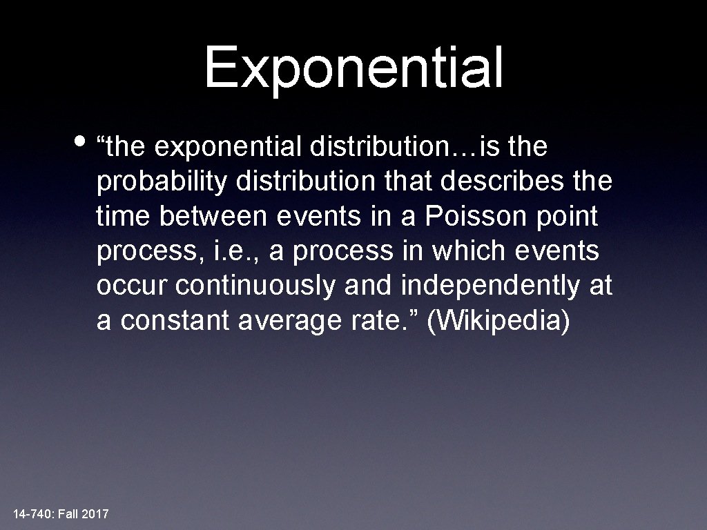
Exponential • “the exponential distribution…is the probability distribution that describes the time between events in a Poisson point process, i. e. , a process in which events occur continuously and independently at a constant average rate. ” (Wikipedia) 14 -740: Fall 2017

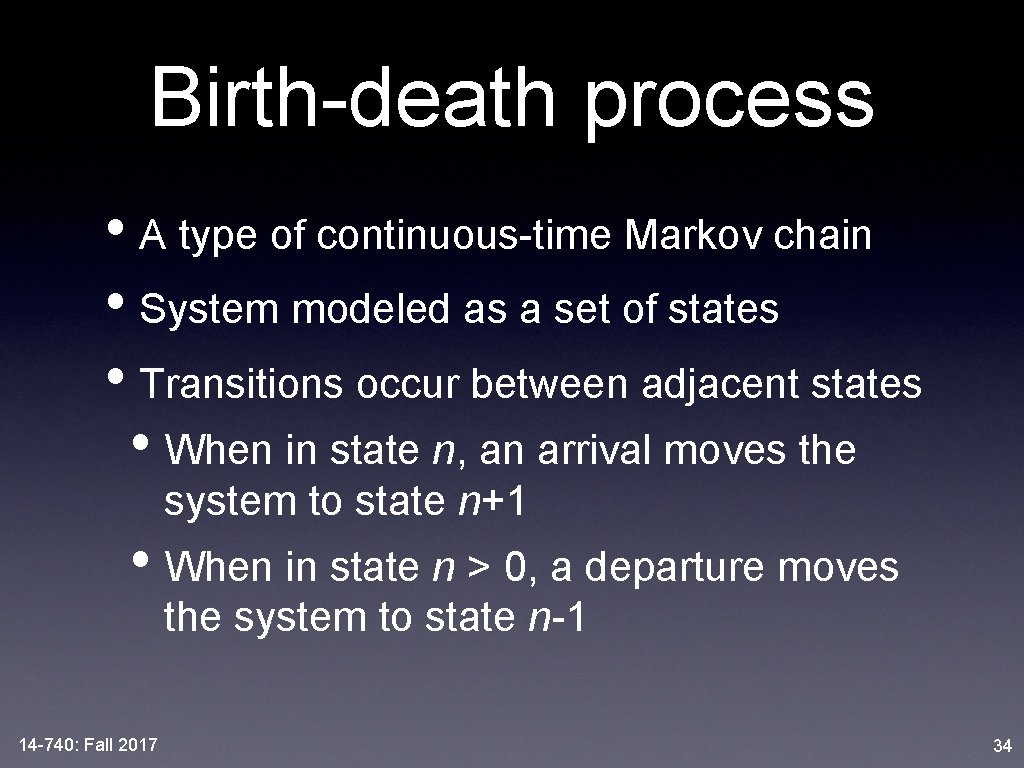
Deterministic • “In mathematics, a degenerate [Deterministic] distribution is a probability distribution in a space (discrete or continuous) with support only on a space of lower dimension. If the degenerate distribution is univariate (involving only a single random variable) it is a deterministic distribution and takes only a single value. Examples include a two-headed coin and rolling a dice whose sides all show the same number. ”(Wikipedia) 14 -740: Fall 2017

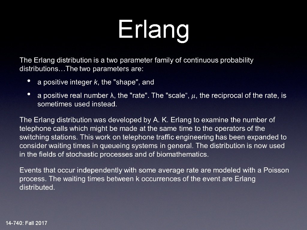
Erlang • 14 -740: Fall 2017

General • Known mean and variance, but nothing else. 14 -740: Fall 2017

Markovian • A Markov chain is "a stochastic model describing a sequence of possible events in which the probability of each event depends only on the state attained in the previous event. " • In probability theory and related fields, a Markov process, named after the Russian mathematician Andrey Markov, is a stochastic process that satisfies the Markov property (Wikipedia) 14 -740: Fall 2017

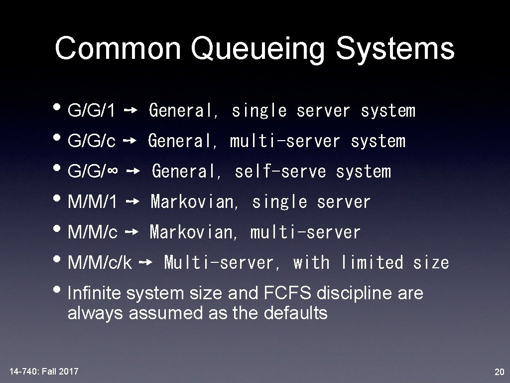
Common Queueing Systems • G/G/1 ➙ General, single server system • G/G/c ➙ General, multi-server system • G/G/∞ ➙ General, self-serve system • M/M/1 ➙ Markovian, single server • M/M/c ➙ Markovian, multi-server • M/M/c/k ➙ Multi-server, with limited size • Infinite system size and FCFS discipline are always assumed as the defaults 14 -740: Fall 2017 20

traceroute • QT Overview • Performance Evaluation • Little’s Law • Rate Transition Diagrams • M/M/1 Systems • M/M/c Systems • Examples 14 -740: Fall 2017 21

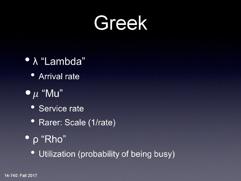
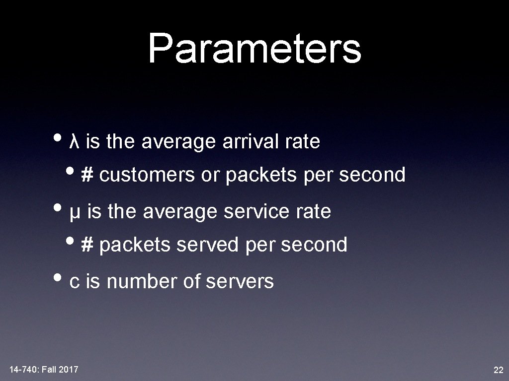
Parameters • λ is the average arrival rate • # customers or packets per second • μ is the average service rate • # packets served per second • c is number of servers 14 -740: Fall 2017 22

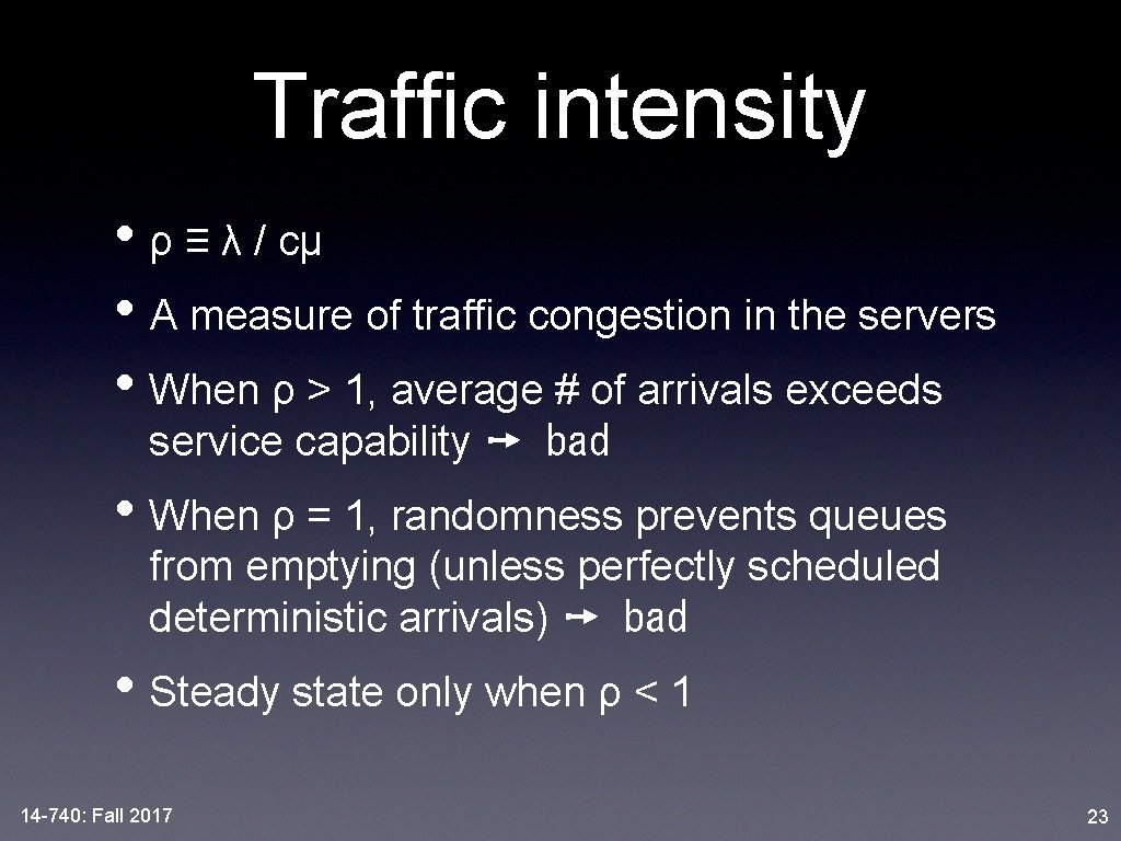
Traffic intensity • ρ ≡ λ / cμ • A measure of traffic congestion in the servers • When ρ > 1, average # of arrivals exceeds service capability ➙ bad • When ρ = 1, randomness prevents queues from emptying (unless perfectly scheduled deterministic arrivals) ➙ bad • Steady state only when ρ < 1 14 -740: Fall 2017 23

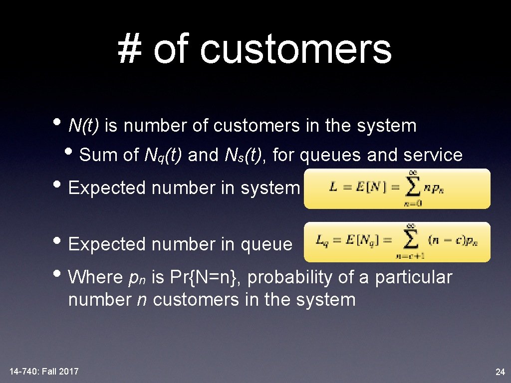
# of customers • N(t) is number of customers in the system • Sum of Nq(t) and Ns(t), for queues and service • Expected number in system • Expected number in queue • Where pn is Pr{N=n}, probability of a particular number n customers in the system 14 -740: Fall 2017 24

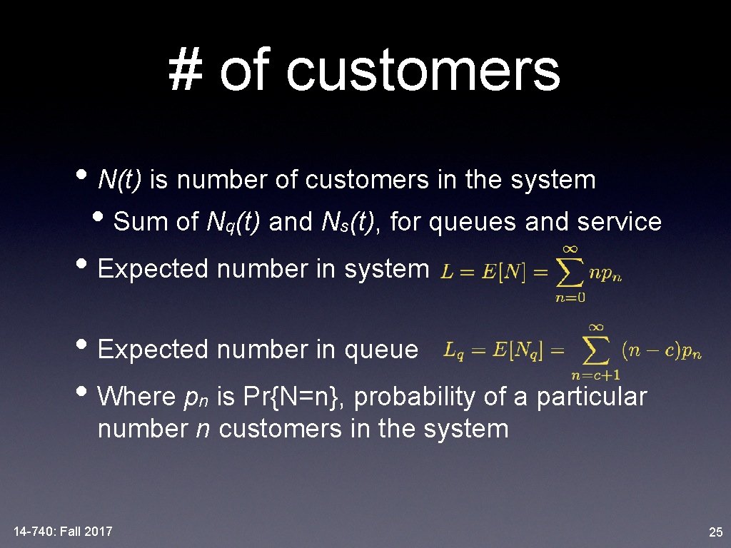
# of customers • N(t) is number of customers in the system • Sum of Nq(t) and Ns(t), for queues and service • Expected number in system • Expected number in queue • Where pn is Pr{N=n}, probability of a particular number n customers in the system 14 -740: Fall 2017 25

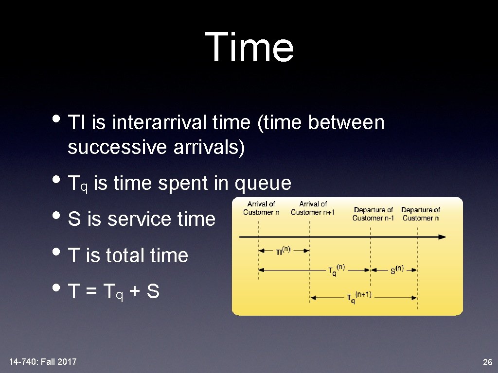
Time • TI is interarrival time (time between successive arrivals) • Tq is time spent in queue • S is service time • T is total time • T = Tq + S 14 -740: Fall 2017 26

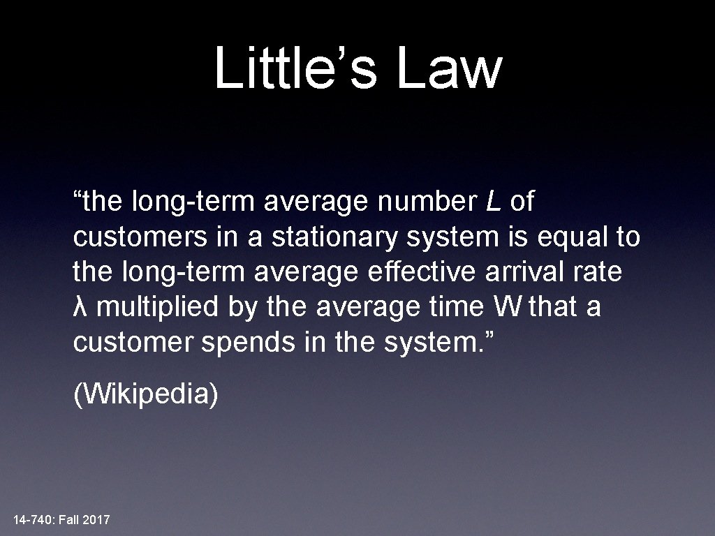
Little’s Law “the long-term average number L of customers in a stationary system is equal to the long-term average effective arrival rate λ multiplied by the average time W that a customer spends in the system. ” (Wikipedia) 14 -740: Fall 2017

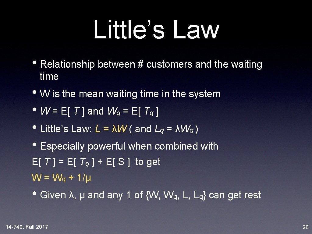
Little’s Law • Relationship between # customers and the waiting time • W is the mean waiting time in the system • W = E[ T ] and Wq = E[ Tq ] • Little’s Law: L = λW ( and Lq = λWq ) • Especially powerful when combined with E[ T ] = E[ Tq ] + E[ S ] to get W = Wq + 1/μ • Given λ, μ and any 1 of {W, Wq, L, Lq} can get rest 14 -740: Fall 2017 28

Further Results • What is E[ Ns ]? • L - Lq = λ(W - Wq) = λ(1/μ) = λ / μ • r ≡ λ / μ • For c=1, r = ρ and 14 -740: Fall 2017 30

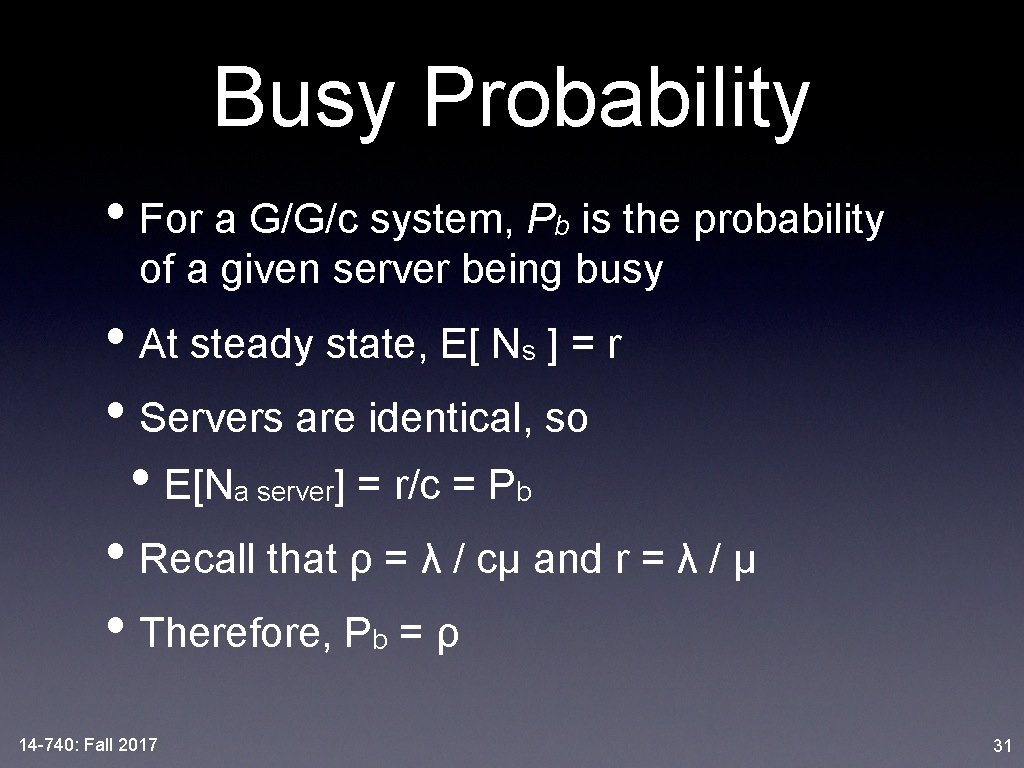
Busy Probability • For a G/G/c system, Pb is the probability of a given server being busy • At steady state, E[ Ns ] = r • Servers are identical, so • E[Na server] = r/c = Pb • Recall that ρ = λ / cμ and r = λ / μ • Therefore, Pb = ρ 14 -740: Fall 2017 31

traceroute • QT Overview • Performance Evaluation • Little’s Law • Rate Transition Diagrams • M/M/1 Systems • M/M/c Systems • Examples 14 -740: Fall 2017 33

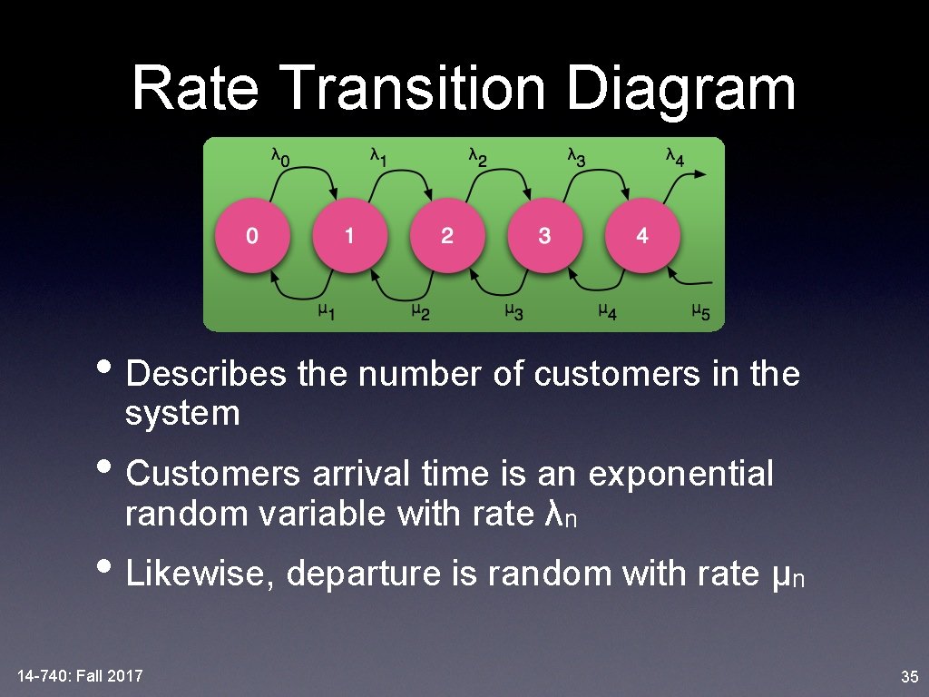
Birth-death process • A type of continuous-time Markov chain • System modeled as a set of states • Transitions occur between adjacent states • When in state n, an arrival moves the system to state n+1 • When in state n > 0, a departure moves the system to state n-1 14 -740: Fall 2017 34

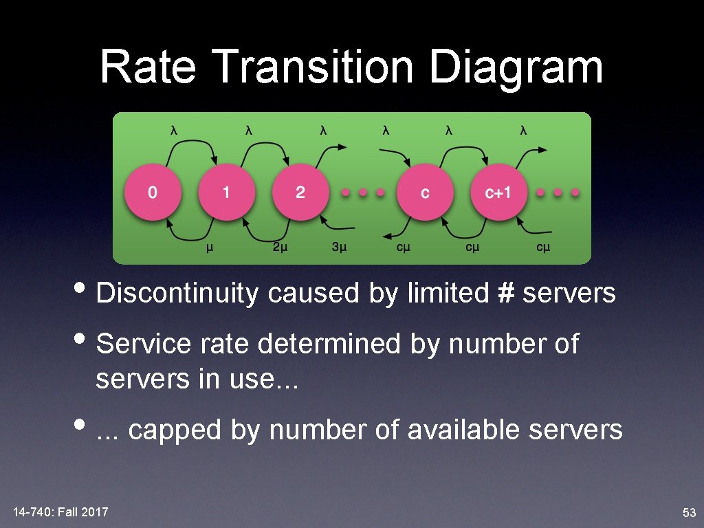
Rate Transition Diagram • Describes the number of customers in the system • Customers arrival time is an exponential random variable with rate λn • Likewise, departure is random with rate μn 14 -740: Fall 2017 35

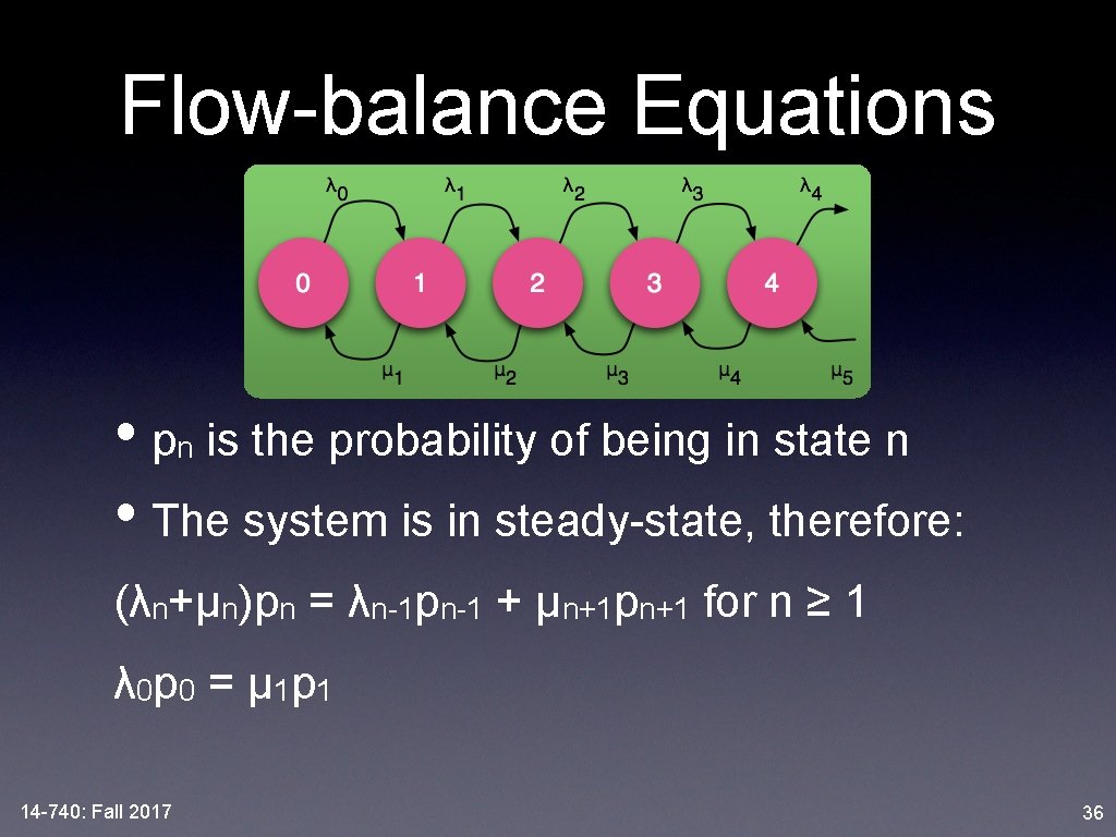
Flow-balance Equations • pn is the probability of being in state n • The system is in steady-state, therefore: (λn+μn)pn = λn-1 pn-1 + μn+1 pn+1 for n ≥ 1 λ 0 p 0 = μ 1 p 1 14 -740: Fall 2017 36

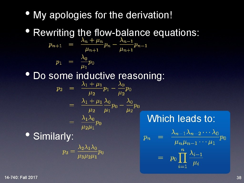
• My apologies for the derivation! • Rewriting the flow-balance equations: • Do some inductive reasoning: Which leads to: • Similarly: 14 -740: Fall 2017 38

traceroute • QT Overview • Performance Evaluation • Little’s Law • Rate Transition Diagrams • M/M/1 Systems • M/M/c Systems • Examples 14 -740: Fall 2017 39

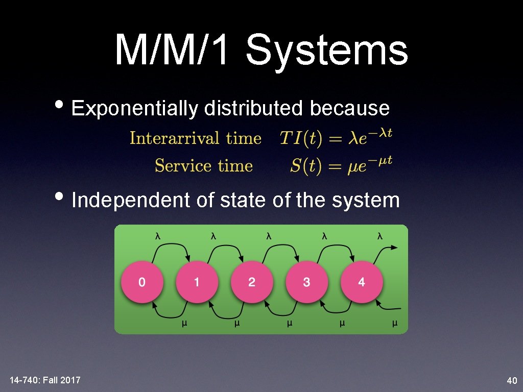
M/M/1 Systems • Exponentially distributed because • Independent of state of the system 14 -740: Fall 2017 40

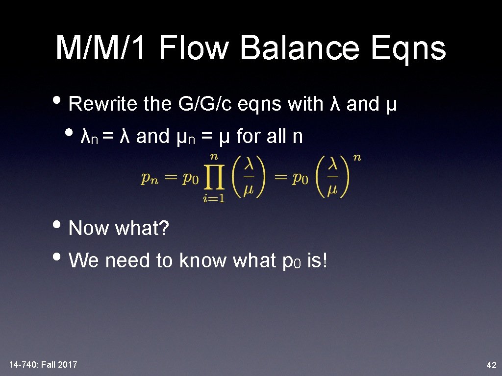
M/M/1 Flow Balance Eqns • Rewrite the G/G/c eqns with λ and μ • λn = λ and μn = μ for all n • Now what? • We need to know what p 0 is! 14 -740: Fall 2017 41

M/M/1 Flow Balance Eqns • Rewrite the G/G/c eqns with λ and μ • λn = λ and μn = μ for all n • Now what? • We need to know what p 0 is! 14 -740: Fall 2017 42

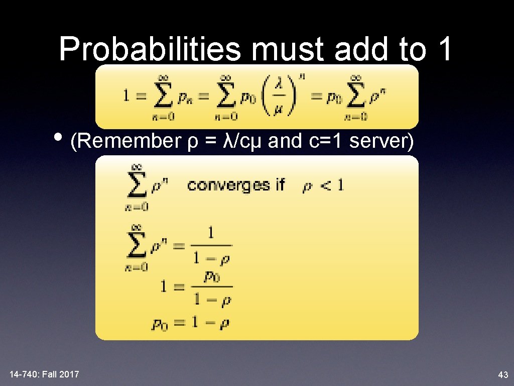
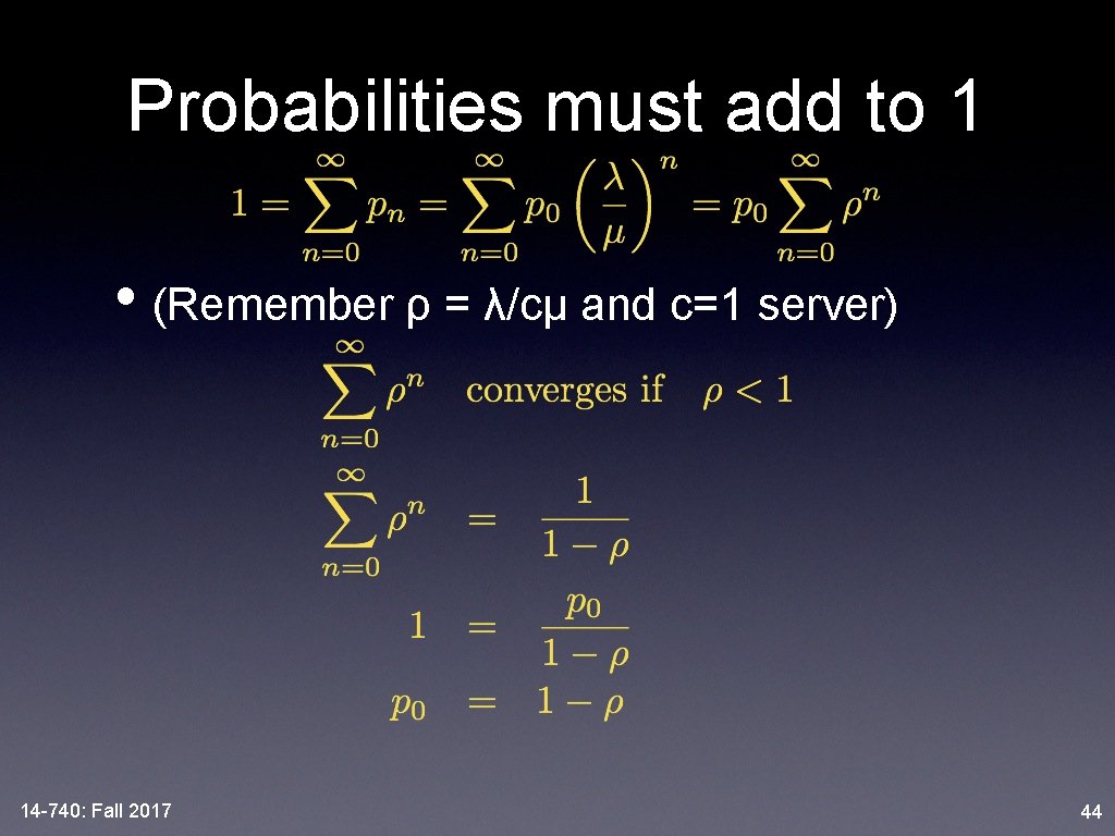
Probabilities must add to 1 • (Remember ρ = λ/cμ and c=1 server) 14 -740: Fall 2017 43

Probabilities must add to 1 • (Remember ρ = λ/cμ and c=1 server) 14 -740: Fall 2017 44

Plug p 0 into Flow-Balance • This final equation is incredibly useful, as it allows us to determine probabilities of system state, given only λ and μ • Also allows us to generate measures of effectiveness 14 -740: Fall 2017 45

Plug p 0 into Flow-Balance • This final equation is incredibly useful, as it allows us to determine probabilities of system state, given only λ and μ • Also allows us to generate measures of effectiveness 14 -740: Fall 2017 46

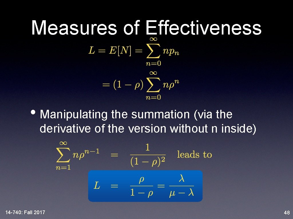
Measures of Effectiveness • Manipulating the summation (via the derivative of the version without n inside) 14 -740: Fall 2017 48

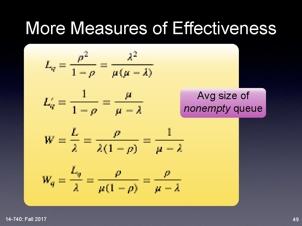
More Measures of Effectiveness Avg size of nonempty queue 14 -740: Fall 2017 49

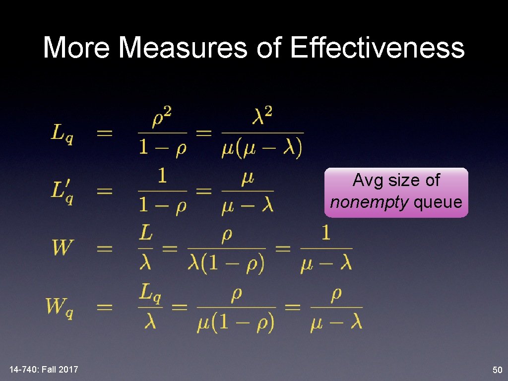
More Measures of Effectiveness Avg size of nonempty queue 14 -740: Fall 2017 50

traceroute • QT Overview • Performance Evaluation • Little’s Law • Rate Transition Diagrams • M/M/1 Systems • M/M/c Systems • Examples 14 -740: Fall 2017 51

M/M/c Systems • How are things different with multiple servers? • Arrival rate is still constant ➙ λ • Service rate is not • System has service capability of cμ • Assuming c customers to service 14 -740: Fall 2017 52

Rate Transition Diagram • Discontinuity caused by limited # servers • Service rate determined by number of servers in use. . . • . . . capped by number of available servers 14 -740: Fall 2017 53

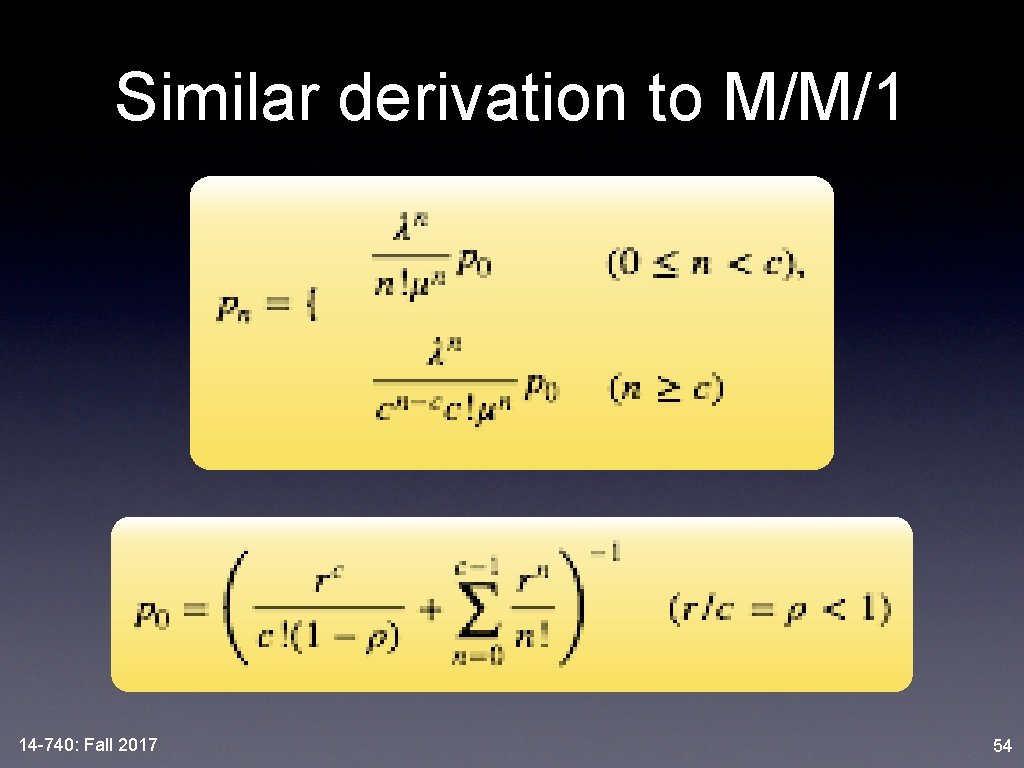
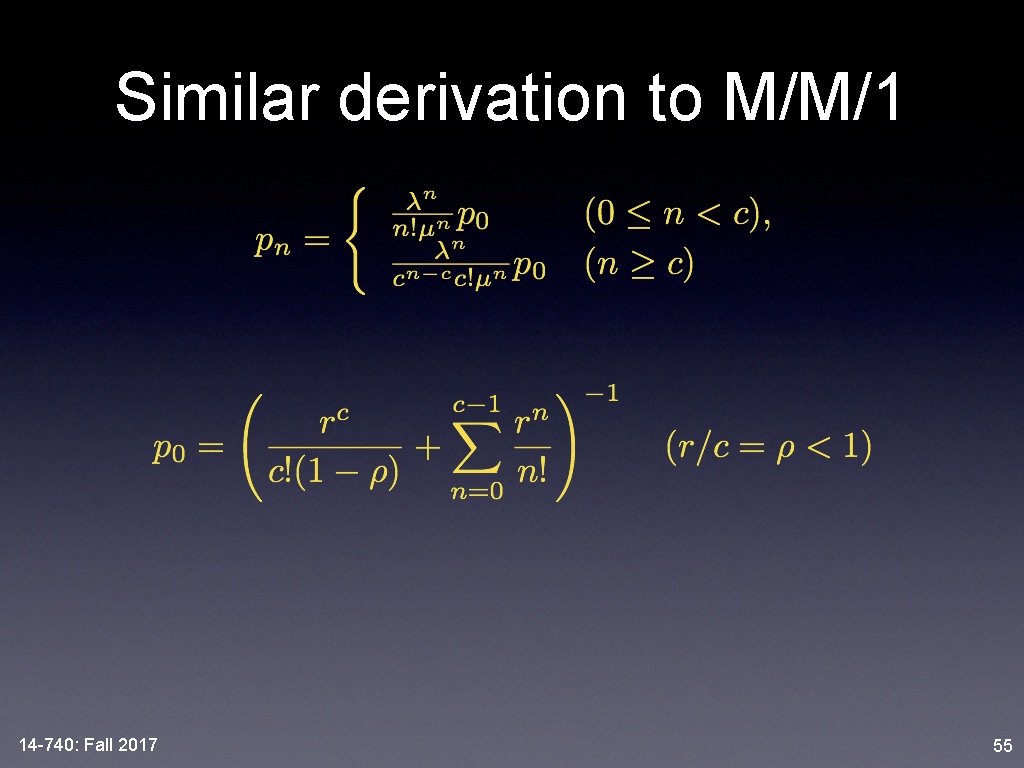
Similar derivation to M/M/1 14 -740: Fall 2017 54

Similar derivation to M/M/1 14 -740: Fall 2017 55

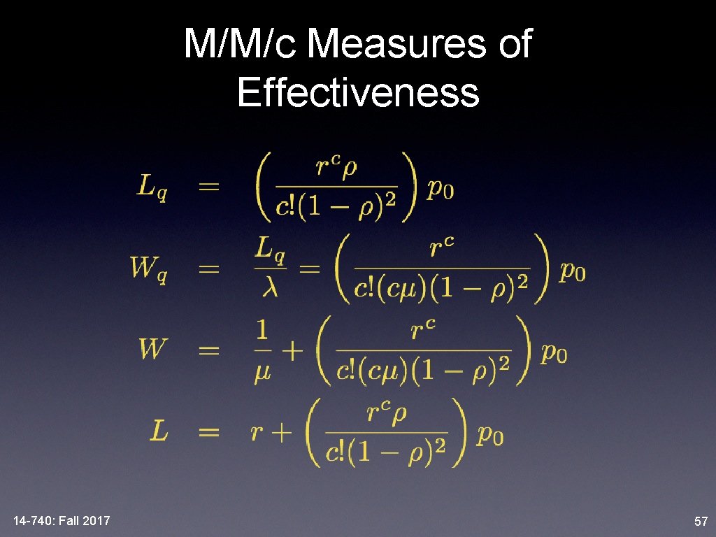
M/M/c Measures of Effectiveness 14 -740: Fall 2017 57

traceroute • QT Overview • Performance Evaluation • Little’s Law • Rate Transition Diagrams • M/M/1 Systems • M/M/c Systems • Examples 14 -740: Fall 2017 58

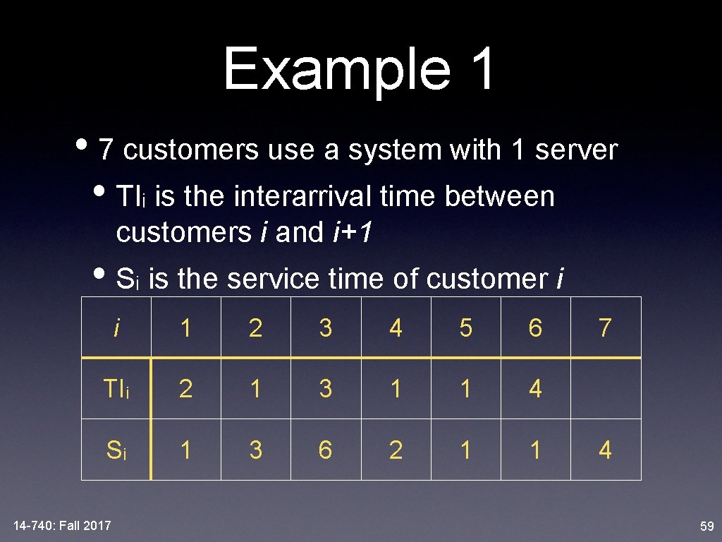
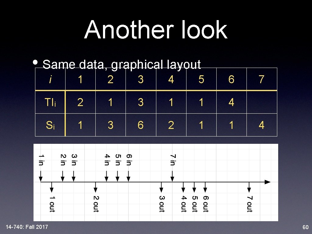
Example 1 • 7 customers use a system with 1 server • TIi is the interarrival time between customers i and i+1 • Si is the service time of customer i i 1 2 3 4 5 6 TIi 2 1 3 1 1 4 Si 1 3 6 2 1 1 14 -740: Fall 2017 7 4 59

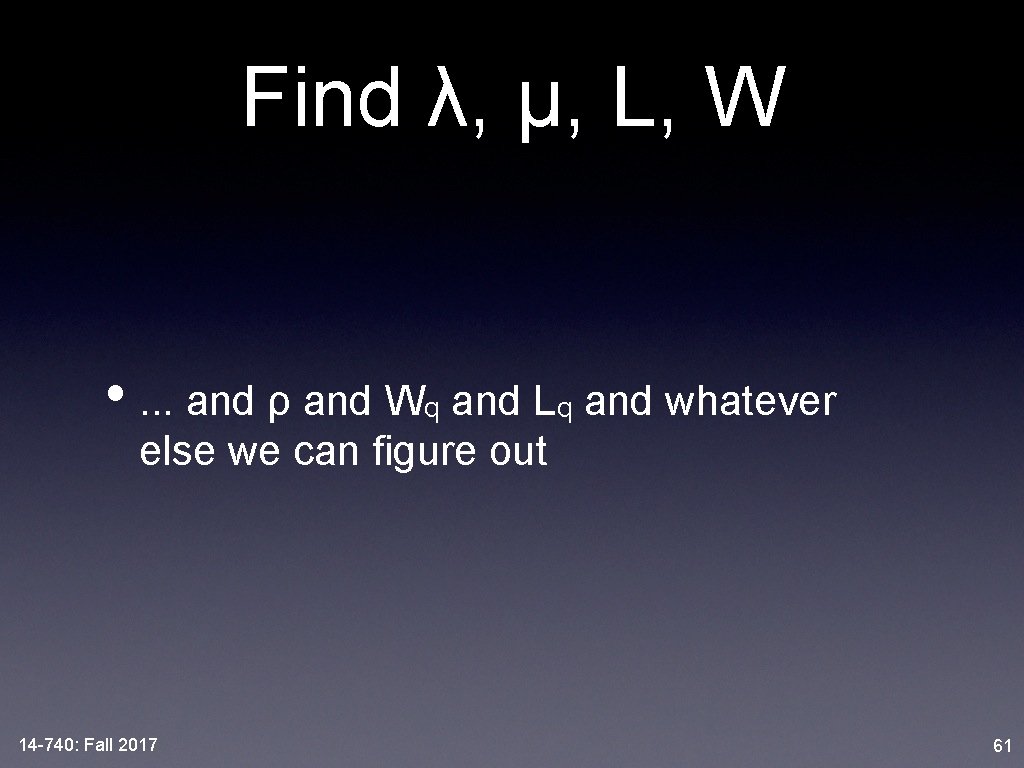
Another look • Same data, graphical layout i 1 2 3 4 5 6 TIi 2 1 3 1 1 4 Si 1 3 6 2 1 1 14 -740: Fall 2017 7 4 60

Find λ, μ, L, W • . . . and ρ and Wq and Lq and whatever else we can figure out 14 -740: Fall 2017 61

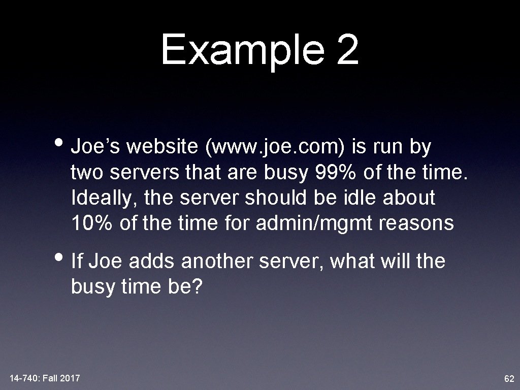
Example 2 • Joe’s website (www. joe. com) is run by two servers that are busy 99% of the time. Ideally, the server should be idle about 10% of the time for admin/mgmt reasons • If Joe adds another server, what will the busy time be? 14 -740: Fall 2017 62

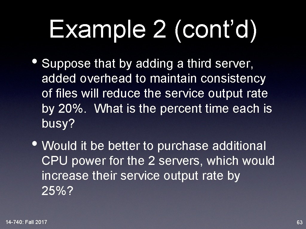
Example 2 (cont’d) • Suppose that by adding a third server, added overhead to maintain consistency of files will reduce the service output rate by 20%. What is the percent time each is busy? • Would it be better to purchase additional CPU power for the 2 servers, which would increase their service output rate by 25%? 14 -740: Fall 2017 63

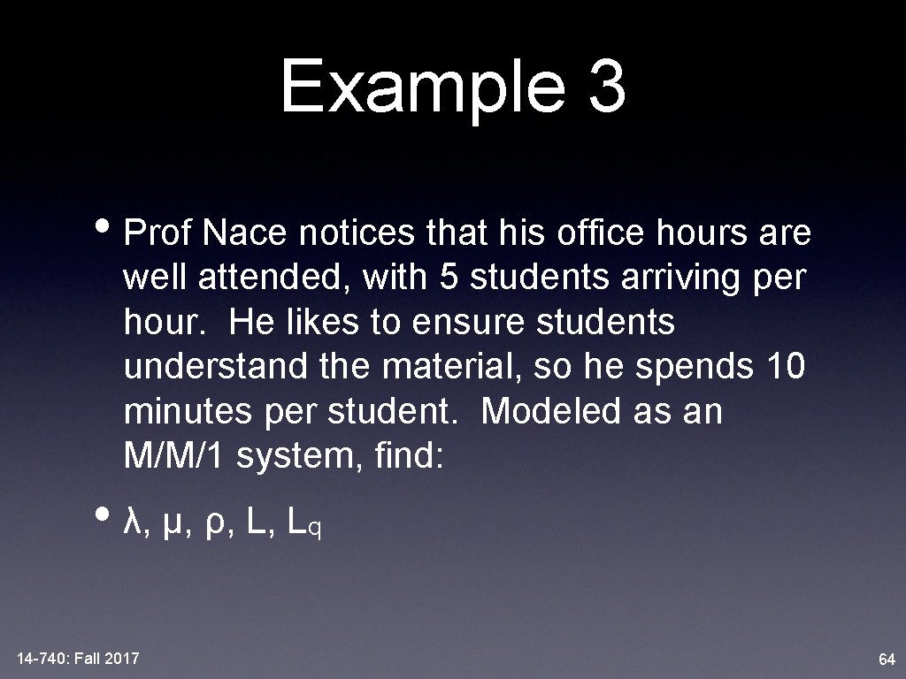
Example 3 • Prof Nace notices that his office hours are well attended, with 5 students arriving per hour. He likes to ensure students understand the material, so he spends 10 minutes per student. Modeled as an M/M/1 system, find: • λ, μ, ρ, L, Lq 14 -740: Fall 2017 64

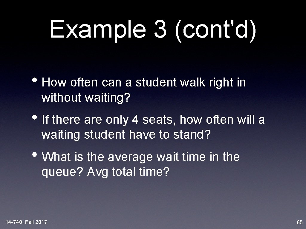
Example 3 (cont'd) • How often can a student walk right in without waiting? • If there are only 4 seats, how often will a waiting student have to stand? • What is the average wait time in the queue? Avg total time? 14 -740: Fall 2017 65

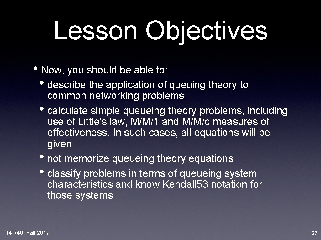
Lesson Objectives • Now, you should be able to: • describe the application of queuing theory to • • • common networking problems calculate simple queueing theory problems, including use of Little's law, M/M/1 and M/M/c measures of effectiveness. In such cases, all equations will be given not memorize queueing theory equations classify problems in terms of queueing system characteristics and know Kendall 53 notation for those systems 14 -740: Fall 2017 67