Python Python https www python orgdownloads Anaconda https

Python程式開發環境 官方版Python https: //www. python. org/downloads Anaconda開發環境 https: //www. anaconda. com/download

Python撰寫 具 官方版IDLE Anaconda Jupyter Notebook 範例檔案放置於：ftp: //163. 25. 117/nplu/Py. Practice

關鍵字 常數 l l l False True None 控制結構 l l l if for … False class finally return None continue for lambda try True def from nonlocal while and del as yield pass raise global elif assert break with or import in not if else except is

流程控制--判斷結構 (Decision Structures) 單向if x=2 y=1 if x > y: z=x-y print("x比y大", z) 雙向if. . . else score = 59 if score >= 60: print("及格！") else: print("不及格！") 多向if. . . else score = 80 if score >= 90: print("優等") elif score < 90 and score >= 80: print("甲等") elif score < 80 and score >= 70: print("乙等") elif score < 70 and score >= 60: print("丙等") else: print("不及格")

流程控制--迴圈結構 (Loop Structures) for var in iterator: statements 1 [else: statements 2] 範例 1: for i in range(5): print(i) 範例 2: list 1 = [15, 20, 33, 7, 8] sum = 0 for i in list 1: sum = sum + i print("總和等於", sum)

流程控制—巢狀迴圈 (Nested Loops) 範例 : 九九乘法表 result 2 = '' for i in range(2, 10): result 1 = '' for j in range(2, 10): result 1 = result 1 + str(i) + '*' + str(j) + '=' + str(i * j) + 't' result 2 = result 2 + result 1 + 'n' print(result 2) 2*2=4 2*3=6 2*4=8 2*5=10 2*6=12 2*7=14 2*8=16 2*9=18 3*2=6 3*3=9 3*4=12 3*5=15 3*6=18 3*7=21 3*8=24 3*9=27 4*2=8 4*3=12 4*4=16 4*5=20 4*6=24 4*7=28 4*8=32 4*9=36 5*2=10 5*3=15 5*4=20 5*5=25 5*6=30 5*7=35 5*8=40 5*9=45 6*2=12 6*3=18 6*4=24 6*5=30 6*6=36 6*7=42 6*8=48 6*9=54 7*2=14 7*3=21 7*4=28 7*5=35 7*6=42 7*7=49 7*8=56 7*9=63 8*2=16 8*3=24 8*4=32 8*5=40 8*6=48 8*7=56 8*8=64 8*9=72 9*2=18 9*3=27 9*4=36 9*5=45 9*6=54 9*7=63 9*8=72 9*9=81

Num. Py統計函式 ü ü ü ü amin(a, axis=None) amax(a, axis=None) nanmin(a, axis=None) average(a, axis=None, weights=None) median(a, axis=None) mean(a, axis=None) std(a, axis=None) var(a, axis=None) nanmedian(a, axis=None) nanmean(a, axis=None) nanstd(a, axis=None) nanvar(a, axis=None) … >>> score = np. array([[80, 75, 88, 80, 78], [88, 86, 90, 95, 86], [92, 85, 92, 98, 90], [81, 88, 80, 82, 85], [75, 80, 78, 80, 70]]) # 算術平均 >>> np. mean(score, axis = 1) array([80. 2, 89. , 91. 4, 83. 2, 76. 6]) # 加權平均 >>> np. average(score, axis = 1, weights = [0. 5, 0. 2, 0. 1, 0. 1]) array([79. 6, 88. 3, 91. , 82. 8, 76. 3]) >>> np. median(score, axis = 1) # 中位數 array([80. , 88. , 92. , 82. , 78. ]) >>> np. std(score, axis = 1) # 標準差 array([4. 30813185, 3. 34664011, 4. 1761226 , 2. 92574777, 3. 77359245]) >>> np. var(score, axis = 1) # 變異數 array([18. 56, 11. 2 , 17. 44, 8. 56, 14. 24])

Num. Py隨機取樣函式 簡單亂數資料 ü ü ü ü ü rand(d 0, d 1, …, dn) randn(d 0, d 1, …, dn) randint(low[, high, size, dtype]) random_integers(low[, high, size]) random_sample([size]) random([size]) ranf([size]) sample([size]) choice(a[, size, replace, p]) 變更順序 ü ü shuffle(x) permutation(x) 亂數�生器 ü seed(seed=None) 分佈 (distribution) ü ü ü ü beta(a, b[, size]) binomial(n, p[, size]) chisquare(df[, size]) dirichlet(alpha[, size]) exponential([scale, size]) f(dfnum, dfden[, size]) gamma(shape[, scale, size]) geometric(p[, size]) gumbel([loc, scale, size]) hypergeometric(ngood, nbad, nsample[, size]) laplace([loc, scale, size]) logistic([loc, scale, size]) lognormal([mean, sigma, size]) ……

常態分佈(n=10000, bins=30) >>> import numpy as np >>> import matplotlib. pyplot as plt >>> samples = np. random. normal(size = 10000) >>> plt. hist(samples, bins = 30) (array([1. 000 e+00, 8. 000 e+00, 5. 000 e+00, 1. 100 e+01, 2. 400 e+01, 5. 800 e+01, 1. 060 e+02, 1. 690 e+02, 2. 400 e+02, 3. 920 e+02, 5. 940 e+02, 7. 220 e+02, 8. 820 e+02, 9. 890 e+02, 1. 052 e+03, 1. 017 e+03, 9. 090 e+02, 8. 420 e+02, 6. 750 e+02, 4. 430 e+02, 3. 270 e+02, 2. 370 e+02, 1. 490 e+02, 7. 000 e+01, 5. 000 e+01, 1. 600 e+01, 6. 000 e+00, 4. 000 e+00, 0. 000 e+00, 2. 000 e+00]), array([-3. 91503377, -3. 64992985, -3. 38482593, -3. 11972202, -2. 8546181 , -2. 58951418, -2. 32441027, -2. 05930635, -1. 79420243, -1. 52909852, -1. 2639946 , -0. 99889068, -0. 73378677, -0. 46868285, -0. 20357893, 0. 06152498, 0. 3266289 , 0. 59173281, 0. 85683673, 1. 12194065, 1. 38704456, 1. 65214848, 1. 9172524 , 2. 18235631, 2. 44746023, 2. 71256415, 2. 97766806, 3. 24277198, 3. 5078759 , 3. 77297981, 4. 03808373]), <a list of 30 Patch objects>) >>> plt. show()

Examples. py程式片段： import math import pandas as pd …. . # data = {'Time': ['2018/4/12 08: 45: 00', '2018/4/12 08: 50: 00 ', '2018/4/12 08: 55: 00'], # 'A. PV - Average': [49. 41580318, 62. 62195005, 62. 02720746], # 'B. OP - Average': [64. 12516777, 63. 6363677999999], # 'C. PV - Average': [56. 11305857, 54. 62703102, 55. 69705158]} # myframe = pd. Data. Frame(data, dtype="float 64" , index=[5, 6, 89]) # Read in dataframe csv. File = "C: /Users/NPLU/Desktop/Py. Practice/input. File. csv" myframe = pd. read_csv(csv. File) print("1. 匯入資料集：") print(myframe. head()) # input file name # LSM from matplotlib import pyplot as plt import numpy as np from sklearn. linear_model import Linear. Regression # x values x = np. array([[45], [50], [55]]) # y values y = np. array(myframe. iloc[: , 1]) 62. 02720746] # A. PV: [49. 41580318, 62. 62195005, n = x. shape[1] r = np. linalg. matrix_rank(x) U, sigma, VT = np. linalg. svd(x, full_matrices=False) myframe. index=[5, 6, 89] D_plus = np. diag(np. hstack([1/sigma[: r], np. zeros(n-r)])) print("n 2. 更動資料集index：") print(myframe. head()) V = VT. T # 標準差 print("n 3. 標準差：") print(myframe. std(axis=0)) # 均方根誤差 dsum = 0 for measured_value in myframe. iloc[: , 1]: dsum = dsum + (myframe. mean()[0] - measured_value)**2 MSE = dsum / 3 RMSE = math. sqrt(MSE) print("n 4. 均方根誤差：") print(RMSE) x_plus = V. dot(D_plus). dot(U. T) w = x_plus. dot(y) plt. scatter(x, y) plt. plot(x, w*x, c='red') print("n 11. LCM結果呈現於圖形視窗中. . . ") plt. show() print("n*** Examples. py執行完畢 ***") …… 完整檔案放置於：ftp: //163. 25. 117/nplu/Py. Practice

創建Pandas資料(手動鍵入) import pandas as pd Data Type: Dict data = {'Time': ['2018/4/12 08: 45: 00', '2018/4/12 08: 50: 00 ', '2018/4/12 08: 55: 00'], 'A. PV - Average': [49. 41580318, 62. 62195005, 62. 02720746], 'B. OP - Average': [64. 12516777, 63. 6363677999999], 'C. PV - Average': [56. 11305857, 54. 62703102, 55. 69705158]} myframe = pd. Data. Frame(data, dtype="float 64" , index=[5, 6, 89]) Data Frame in Pandas

創建Pandas資料(檔案匯入) import pandas as pd csv. File = "C: /Users/NPLU/Desktop/Py. Practice/input. File. csv " # input file name myframe = pd. read_csv(csv. File) myframe. head() myframe. index=[5, 6, 89] myframe. head() # 改變索引�

標準差之函式呼叫 公式 使用pandas std函式 print(myframe. std()) A. PV B. OP C. PV dtype: Average float 64 7. 458815 0. 282209 0. 766625

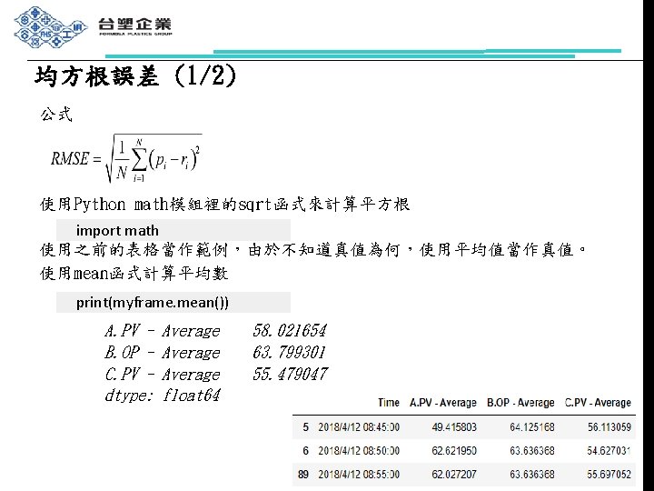
均方根誤差 (2/2) 計算A. PV的均方根誤差 dsum = 0 for measured_value in myframe. iloc[: , 1]: dsum = dsum + pow(myframe. mean()[0] - measured_value, 2) MSE = dsum / 3 RMSE = math. sqrt(MSE) print(RMSE) 6. 090097169576682

變異係數 公式 使用之前的表格當作範例 計算B. OP的變異係數 print(myframe. std()[1] / myframe. mean()[1]) 0. 004423383787761082

變異數 公式 使用之前的表格當作範例 計算A. PV的變異數 dsum = 0 for measured_value in myframe. iloc[: , 1]: dsum = dsum + pow(measured_value - myframe. mean()[0], 2) Var = dsum / 3 print(Var) 37. 08928353488591 import numpy as np print(np. var(myframe. iloc[: , 1])) print(myframe. var(axis=0))

共變異數 公式 使用之前的表格當作範例 計算A. PV和B. OP的共變異數 dsum = 0 for index in range(3): dsum = dsum + ((myframe. iloc[index, 1] - myframe. mean()[0]) * (myframe. iloc[index, 2] - myframe. mean()[1])) Cov = dsum / 3 print(Cov) -1. 4021798030662331

相關係數 公式 使用之前的表格當作範例 計算A. PV和B. OP的相關係數 dsum = 0 for index in range(3): dsum = dsum + ((myframe. iloc[index, 1] - myframe. mean()[0]) * (myframe. iloc[index, 2] - myframe. mean()[1])) Cor = dsum / myframe. std()[0] * myframe. std()[1] print(Cor) -0. 1591569667502748

主成分分析 (Princial Component Analysis, PCA) from sklearn import decomposition pca = decomposition. PCA(n_components=3) pc = pca. fit_transform(myframe. iloc[: , 1: 4]) pc_df = pd. Data. Frame(data = pc, columns = ['PC 1', 'PC 2', 'PC 3']) pc_df. head() pc_df. to_csv(“C: /Users/NPLU/Desktop/Py. Practice/out. PCA. csv”) # out. File https: //cmdlinetips. com/2018/03/pca-example-in-python-with-scikit-learn/

最小平方法(Least Squares Method) • 使用pandas表格之A. PV - Average作範例 from matplotlib import pyplot as plt import numpy as np from sklearn. linear_model import Linear. Regression # x values x = np. array([[45], [50], [55]]) # y values y = np. array(myframe. iloc[: , 1]) # [49. 41580318, 62. 62195005, 62. 02720746] n = x. shape[1] r = np. linalg. matrix_rank(x) U, sigma, VT = np. linalg. svd(x, full_matrices=False) D_plus = np. diag(np. hstack([1/sigma[: r], np. zeros(n-r)])) V = VT. T x_plus = V. dot(D_plus). dot(U. T) w = x_plus. dot(y) plt. scatter(x, y) plt. plot(x, w*x, c='red') plt. show() https: //towardsdatascience. com/least-squares-linear-regression-in-python-54 b 87 fc 49 e 77

參考資料 n Ø Ø n Ø n Ø Python安裝程序 官方版：https: //www. youtube. com/watch? v=wq. Rl. KVRUV_k Anaconda開發環境：https: //www. youtube. com/watch? v=9 LEwsk 8 d. R 3 o Python程式設計 陳惠貞，「一步到位！Python程式設計」，旗標，2019。 主成分分析 https: //cmdlinetips. com/2018/03/pca-example-in-python-with-scikit-learn 最小平方法 https: //towardsdatascience. com/least-squares-linear-regression-in-python 54 b 87 fc 49 e 77

本單元相關檔案 Ø 匯入之套件 Ø Examples. py import pandas import numpy Ø 資料輸入檔 input. File. csv Import matplotlib import sklearn 程式檔 Ø PCA輸出檔 out. PCA. csv Ø Juypter Notebook Examples. ipynb 本單元檔案均放置於：ftp: //163. 25. 117/nplu/Py. Practice