Python IDLE Anaconda Jupyter Notebook Decision Structures if


Python撰寫 具 官方版IDLE Anaconda Jupyter Notebook
 單向if x=2 y=1 if x > y: z=x-y print(\"x比y大\", z) 雙向if.")
流程控制--判斷結構 (Decision Structures) 單向if x=2 y=1 if x > y: z=x-y print("x比y大", z) 雙向if. . . else score = 59 if score >= 60: print("及格!") else: print("不及格!") 多向if. . . else score = 80 if score >= 90: print("優等") elif score < 90 and score >= 80: print("甲等") elif score < 80 and score >= 70: print("乙等") elif score < 70 and score >= 60: print("丙等") else: print("不及格")
![流程控制--迴圈結構 (Loop Structures) for var in iterator: statements 1 [else: statements 2] 範例 1:](http://slidetodoc.com/presentation_image_h2/4b6ed6dca82f225dbf0944dc2a8e5cdf/image-11.jpg "流程控制--迴圈結構 (Loop Structures) for var in iterator: statements 1 [else: statements 2] 範例 1:")
流程控制--迴圈結構 (Loop Structures) for var in iterator: statements 1 [else: statements 2] 範例 1: for i in range(5): print(i) 範例 2: list 1 = [15, 20, 33, 7, 8] sum = 0 for i in list 1: sum = sum + i print("總和等於", sum)
 amax(a, axis=None) nanmin(a, axis=None) average(a, axis=None,")
Num. Py統計函式 ü ü ü ü amin(a, axis=None) amax(a, axis=None) nanmin(a, axis=None) average(a, axis=None, weights=None) median(a, axis=None) mean(a, axis=None) std(a, axis=None) var(a, axis=None) nanmedian(a, axis=None) nanmean(a, axis=None) nanstd(a, axis=None) nanvar(a, axis=None) … >>> score = np. array([[80, 75, 88, 80, 78], [88, 86, 90, 95, 86], [92, 85, 92, 98, 90], [81, 88, 80, 82, 85], [75, 80, 78, 80, 70]]) # 算術平均 >>> np. mean(score, axis = 1) array([80. 2, 89. , 91. 4, 83. 2, 76. 6]) # 加權平均 >>> np. average(score, axis = 1, weights = [0. 5, 0. 2, 0. 1, 0. 1]) array([79. 6, 88. 3, 91. , 82. 8, 76. 3]) >>> np. median(score, axis = 1) array([80. , 88. , 92. , 82. , 78. ]) # 中位數 >>> np. std(score, axis = 1) # 標準差 array([4. 30813185, 3. 34664011, 4. 1761226 , 2. 92574777, 3. 77359245])
 import numpy as np import matplotlib. pyplot as plt samples = np.")
標準常態分佈(n=10000, bins=30) import numpy as np import matplotlib. pyplot as plt samples = np. random. normal(size = 10000) plt. hist(samples, bins = 30) plt. show()

 import pandas as pd Data Type: Dict data = {'Time': ['2018/4/12 08: 45',")
創建Pandas資料(手動鍵入) import pandas as pd Data Type: Dict data = {'Time': ['2018/4/12 08: 45', '2018/4/12 08: 50 ', '2018/4/12 08: 55'], 'A': [49. 4, 62. 6, 62. 0], 'B': [64. 1, 63. 6], 'C': [56. 1, 54. 6, 55. 7]} myframe = pd. Data. Frame(data, dtype="float 64" , index=[5, 6, 89]) Data Frame in Pandas
 import pandas as pd csv. File = \"C: /Users/User/Desktop/Py. Practice/in. File. csv \"")
創建Pandas資料(檔案匯入) import pandas as pd csv. File = "C: /Users/User/Desktop/Py. Practice/in. File. csv " # input file name myframe = pd. read_csv(csv. File) myframe. head() myframe. index=[5, 6, 89] # 改變索引� myframe. head()
) A 7. 453858 B 0. 288675 C 0.")
標準差之函式呼叫 公式 使用pandas std函式 print(myframe. std()) A 7. 453858 B 0. 288675 C 0. 776745 dtype: float 64
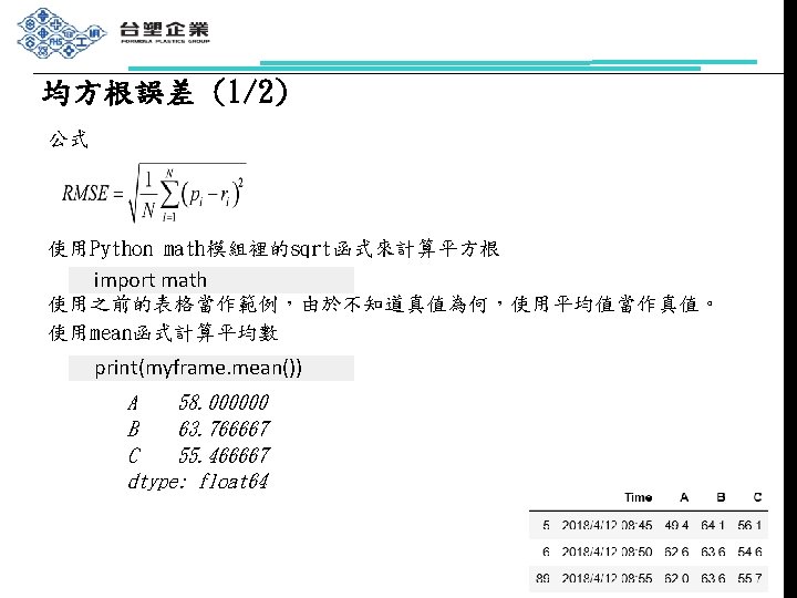
![均方根誤差 (2/2) 計算欄位A的均方根誤差 dsum = 0 for measured_value in myframe. iloc[: , 1]: dsum](http://slidetodoc.com/presentation_image_h2/4b6ed6dca82f225dbf0944dc2a8e5cdf/image-20.jpg "均方根誤差 (2/2) 計算欄位A的均方根誤差 dsum = 0 for measured_value in myframe. iloc[: , 1]: dsum")
均方根誤差 (2/2) 計算欄位A的均方根誤差 dsum = 0 for measured_value in myframe. iloc[: , 1]: dsum = dsum + pow(myframe. mean()[0] - measured_value, 2) MSE = dsum / myframe. iloc[: , 1]. size RMSE = math. sqrt(MSE) print(RMSE) 6. 086049621881177
![變異係數 公式 使用之前的表格當作範例 計算欄位B的變異係數 print(myframe. std()[1] / myframe. mean()[1]) 0. 004527053861915455](http://slidetodoc.com/presentation_image_h2/4b6ed6dca82f225dbf0944dc2a8e5cdf/image-21.jpg "變異係數 公式 使用之前的表格當作範例 計算欄位B的變異係數 print(myframe. std()[1] / myframe. mean()[1]) 0. 004527053861915455")
變異係數 公式 使用之前的表格當作範例 計算欄位B的變異係數 print(myframe. std()[1] / myframe. mean()[1]) 0. 004527053861915455

變異數 公式 使用之前的表格當作範例 計算A. PV的變異數 dsum = 0 for measured_value in myframe. iloc[: , 1]: dsum = dsum + pow(measured_value - myframe. mean()[0], 2) Var = dsum / myframe. iloc[: , 1]. size print(Var) 37. 040000001 import numpy as np print(np. var(myframe. iloc[: , 1])) print(myframe. var(axis=0))
![共變異數 公式 使用之前的表格當作範例 計算欄位A和欄位B的共變異數 dsum = 0 for index in range(myframe. iloc[: , 1].](http://slidetodoc.com/presentation_image_h2/4b6ed6dca82f225dbf0944dc2a8e5cdf/image-23.jpg "共變異數 公式 使用之前的表格當作範例 計算欄位A和欄位B的共變異數 dsum = 0 for index in range(myframe. iloc[: , 1].")
共變異數 公式 使用之前的表格當作範例 計算欄位A和欄位B的共變異數 dsum = 0 for index in range(myframe. iloc[: , 1]. size): dsum = dsum + ((myframe. iloc[index, 1] - myframe. mean()[0]) * (myframe. iloc[index, 2] - myframe. mean()[1])) Cov = dsum / myframe. iloc[: , 1]. size print(Cov) -1. 4333333131
![相關係數 公式 使用之前的表格當作範例 計算A和B的相關係數 dsum = 0 for index in range(myframe. iloc[: , 1].](http://slidetodoc.com/presentation_image_h2/4b6ed6dca82f225dbf0944dc2a8e5cdf/image-24.jpg "相關係數 公式 使用之前的表格當作範例 計算A和B的相關係數 dsum = 0 for index in range(myframe. iloc[: , 1].")
相關係數 公式 使用之前的表格當作範例 計算A和B的相關係數 dsum = 0 for index in range(myframe. iloc[: , 1]. size): dsum = dsum + ((myframe. iloc[index, 1] - myframe. mean()[0]) * (myframe. iloc[index, 2] - myframe. mean()[1])) Cor = dsum / myframe. std()[0] * myframe. std()[1] print(Cor) -0. 16653162275522396
 from sklearn import decomposition pca = decomposition. PCA(n_components=3) pc")
主成分分析 (Princial Component Analysis, PCA) from sklearn import decomposition pca = decomposition. PCA(n_components=3) pc = pca. fit_transform(myframe. iloc[: , 1: 4]) pc_df = pd. Data. Frame(data = pc, columns = ['PC 1', 'PC 2', 'PC 3']) pc_df. head() pc_df. to_csv("out. PCA. csv") # output file name https: //cmdlinetips. com/2018/03/pca-example-in-python-with-scikit-learn/
 • 使用pandas表格之欄位A作範例 from matplotlib import pyplot as plt import numpy as")
最小平方法(Least Squares Method) • 使用pandas表格之欄位A作範例 from matplotlib import pyplot as plt import numpy as np from sklearn. linear_model import Linear. Regression # x values x = np. array([[45], [50], [55]]) # y values y = np. array(myframe. iloc[: , 1]) # [49. 4, 62. 6, 62. 0] n = x. shape[1] r = np. linalg. matrix_rank(x) U, sigma, VT = np. linalg. svd(x, full_matrices=False) D_plus = np. diag(np. hstack([1/sigma[: r], np. zeros(n-r)])) V = VT. T x_plus = V. dot(D_plus). dot(U. T) w = x_plus. dot(y) plt. scatter(x, y) plt. plot(x, w*x, c='red') plt. show() https: //towardsdatascience. com/least-squares-linear-regression-in-python-54 b 87 fc 49 e 77

參考資料 n Ø Ø n Ø n Ø Python安裝程序 官方版:https: //www. youtube. com/watch? v=wq. Rl. KVRUV_k Anaconda開發環境:https: //www. youtube. com/watch? v=9 LEwsk 8 d. R 3 o Python程式設計 陳惠貞,「一步到位!Python程式設計」,旗標,2019。 主成分分析 https: //cmdlinetips. com/2018/03/pca-example-in-python-with-scikit -learn 最小平方法 https: //towardsdatascience. com/least-squares-linear-regression-in -python-54 b 87 fc 49 e 77

本單元需安裝之套件 pip install pandas pip install numpy pip install matplotlib pip install sklearn
- Slides: 28