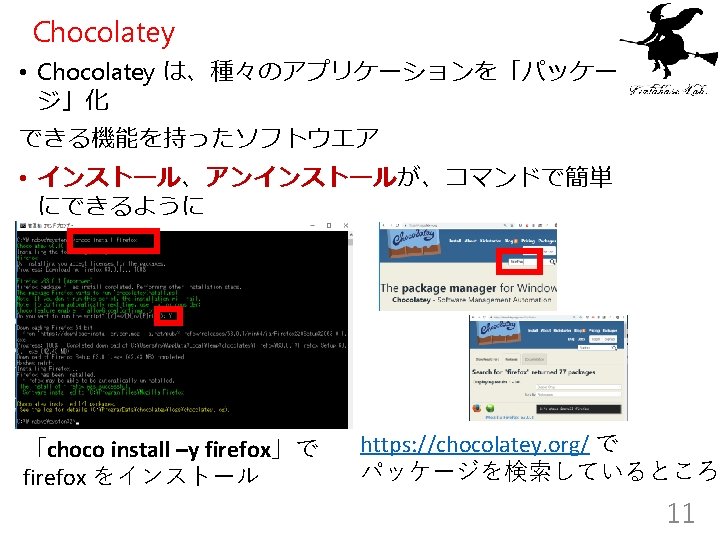
Chocolatey 1 Web Chocolatey Web https chocolatey org


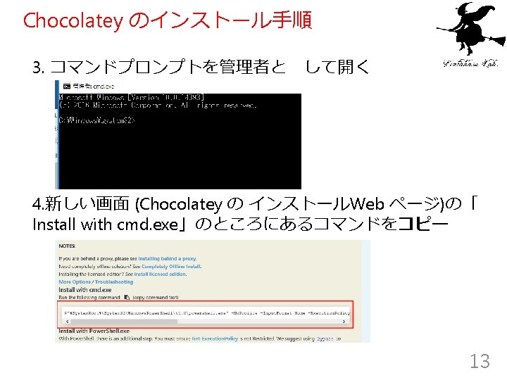
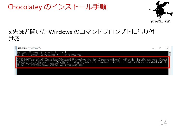
Chocolatey のインストール手順 1. Web ブラウザで、Chocolatey の Web ページを開く https: //chocolatey. org/ 2. 「Install Chocolatey Now」をクリック 12

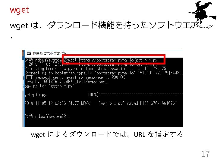
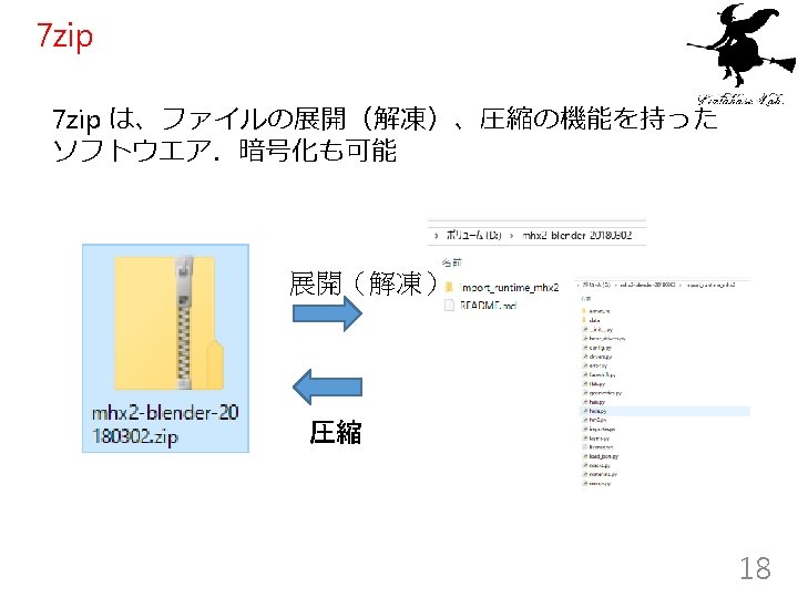
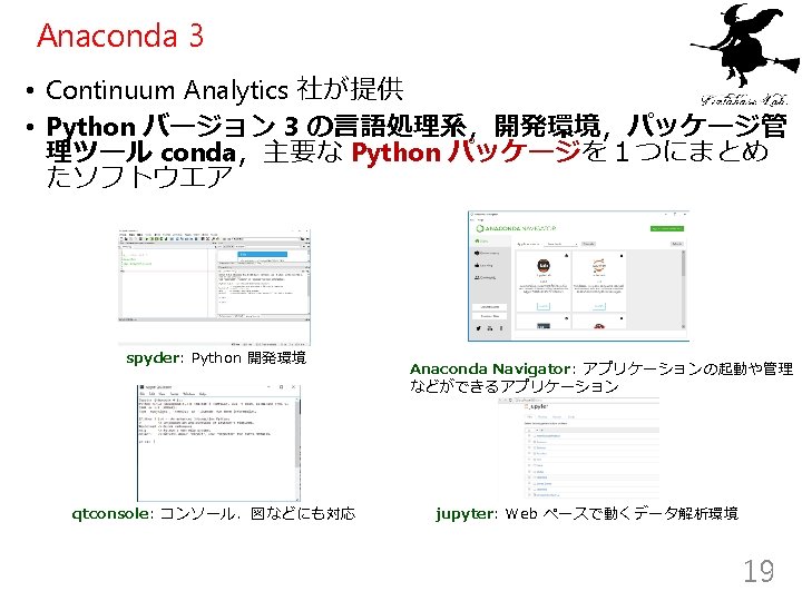
• • • • • • • Chotolatey でパッケージ化されたアプリケー ションの例 ツール: git, cmake, wget, 7 zip Python プログラム開発環境: Anaconda 3, Python 2 Chocolatey の GUI: Chocolatey. GUI ファイル、ストレージ用ツール: Everything, rufus, etcher, sdformatter エディタ: emacs, notepad++, geany Web ブラウザ: Firefox, Google Chrome ネットワークツール: mobaxterm, File. Zilla (ファイル転送), Wireshark (ネットワーク), AWS Command Line Interface (AWS), Google Earth, Real. VNCViewer (リモート接続) 各種ツール類:Paint. NET, Graphviz (グラフデータ構造可視化), Adobe Reader DC (PDF), Git. Hub Desktop, HWi. NFO (ハードウエア情報) Python プログラム開発環境: nteract, ironpython Java JDK 8, Apache Ant Java 関連: Blue. J, Java 開発環境 Eclipse Android: Android Studio, Android SDK Java. Script: Node. js, yarn R システム: Microsoft R Open, RStudio GNU Octave Strawberry Perl Docker: Docker CE (Community Edition) データベース管理システム: SQLite 3, DB Browser for SQLite (sqlitebrowser), Redis 64 bit 3次元コンピュータグラフィックス: Blender, POV-ray, Mesh. Lab, Make. Human グラフィックス、ペイント: Inkscape, GIMP 画像、ビデオ、音声用ツール: imagemagick, FFMpeg, winff, VLC media player (メディア), Openshot, K-Lite Codec Pack Full 設計: Free. CAD ゲームフレームワーク,ゲームエンジン: Unity, Unity Standard Assets, Unity Linux Target Support, Unity i. OS Target Suport, Unity Android Target Suport llvm MSYS 2 15

インターネットのファイルと URL https: //www. kunihikokaneko. com/a/ai. html HTML 形式の Web ページ https: //bootstrap. pypa. io/get-pip. py プログラムファイル 16
、データフローグラフによる数値 演算の機能 import tensorflow as")
Tenfor. Flow • Google 社が公開しているソフトウエア • Python のパッケージ • テンソル(多次元の配列)、データフローグラフによる数値 演算の機能 import tensorflow as tf matrix 1 = tf. constant([[3. , 3. ]]) matrix 2 = tf. constant([[2. ], [2. ]]) product = tf. matmul(matrix 1, matrix 2) sess = tf. Session() result = sess. run(product) print(result) sess. close() 3× 2 + 3× 2 22
が簡単に できるソフトウエア import sklearn. datasets import sklearn. model_selection import keras. utils")
Keras は AI の記述(学習の仕方、応用の仕方)が簡単に できるソフトウエア import sklearn. datasets import sklearn. model_selection import keras. utils import numpy as np iris = sklearn. datasets. load_iris() X = iris. data y = iris. target X_train, X_test, y_train, y_test = sklearn. model_selection. train_test_split(X, y, train_size=0. 5) # 2次元の配列. 要素は float 64, 最大値と最小値を用いて正規化 def normalizer(A): M = np. reshape(A, (len(A), -1)) M = M. astype('float 32') max = M. max(axis=0) min = M. min(axis=0) return (M - min)/(max - min) X_train = normalizer(X_train) X_test = normalizer(X_test) # one-hot y_train = keras. utils. to_categorical(y_train) y_test = keras. utils. to_categorical(y_test) import tensorflow as tf import keras from keras. models import Sequential m = Sequential() from keras. layers import Dense, Activation m. add(Dense(units=64, input_dim=len(X_train[0]))) m. add(Activation('relu')) m. add(Dense(units=3)) m. add(Activation('softmax')) m. compile(loss=keras. losses. categorical_crossentropy, optimizer=keras. optimizers. SGD(lr=0. 01, momentum=0. 9, nesterov=True), metrics=['accuracy']) m. fit(X_train, y_train, batch_size=32, epochs=10, validation_data=(X_test, y_test)) 23
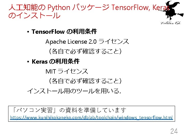
 Anaconda がインストール済み Youtube ビデオ「p-6. Anaconda を Windows マシンにインストール」 https:")
Tensor. Flow, Keras のインストール (前準備) Anaconda がインストール済み Youtube ビデオ「p-6. Anaconda を Windows マシンにインストール」 https: //www. youtube. com/watch? v=Abi. Erivs. IEY 1.Anaconda の conda パッケージの更新、古い conda パ ッケージファイルの削除 conda info conda config --remove channels conda-forge conda upgrade --all conda clean –-packages 2.conda を用いて Tensor. Flow と Keras をインストール conda install -y tensorflow conda install –y keras conda list 25

Open. CV • Open. CV はコンピュータビジョンのソフトウエア • Python からも利用可能 トラッキングビジョンの例 オプティカルフローの例 import cv 2 import numpy as np v = cv 2. Video. Capture("E: /00008. MTS") fourcc = cv 2. Video. Writer_fourcc(*'XVID') while(v. is. Opened()): r, f = v. read() g = cv 2. cvt. Color(f, cv 2. COLOR_BGR 2 GRAY) d = cv 2. good. Features. To. Track(g, 80, 0. 01, 5, 3) if d is not None: d = np. int 0(d) for i in d: x, y = i. ravel() cv 2. circle(f, (x, y), 10, 255, -1) cv 2. imshow("", f) if cv 2. wait. Key(1) & 0 x. FF == ord('q'): break v. release() cv 2. destroy. All. Windows() import cv 2 import numpy as np cap = cv 2. Video. Capture("E: /00008. MTS") fourcc = cv 2. Video. Writer_fourcc(*'XVID') ret, frame 1 = cap. read() prvs = cv 2. cvt. Color(frame 1, cv 2. COLOR_BGR 2 GRAY) hsv = np. zeros_like(frame 1) hsv[. . . , 1] = 255 while(1): ret, frame 2 = cap. read() next = cv 2. cvt. Color(frame 2, cv 2. COLOR_BGR 2 GRAY) # pyr_scale, levels, winsize, iterations, poly_n, poly_sigma, flags flow = cv 2. calc. Optical. Flow. Farneback(prvs, next, None, 0. 5, 3, 15, 3, 5, 1. 2, 0) mag, ang = cv 2. cart. To. Polar(flow[. . . , 0], flow[. . . , 1]) hsv[. . . , 0] = ang*180/np. pi/2 hsv[. . . , 2] = cv 2. normalize(mag, None, 0, 255, cv 2. NORM_MINMAX) rgb = cv 2. cvt. Color(hsv, cv 2. COLOR_HSV 2 BGR) cv 2. imshow('source', frame 2) cv 2. imshow('flow', rgb) if cv 2. wait. Key(1) & 0 x. FF == ord('q'): break prvs = next cap. release() cv 2. destroy. All. Windows() 26

- Slides: 27