Projections and Coordinate Systems Overview Projections Examples of

Projections and Coordinate Systems Overview Projections Examples of different projections Coordinate systems Datums

Projections 2

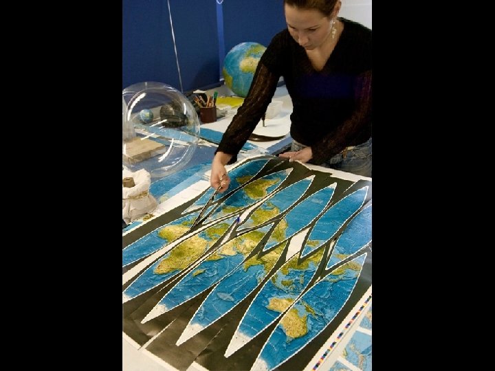
The earth is a spheroid The best model of the earth is a globe Drawbacks: • not easy to carry • not good for making planimetric measurement (distance, area, angle)

Maps are flat easy to carry good for measurement scaleable

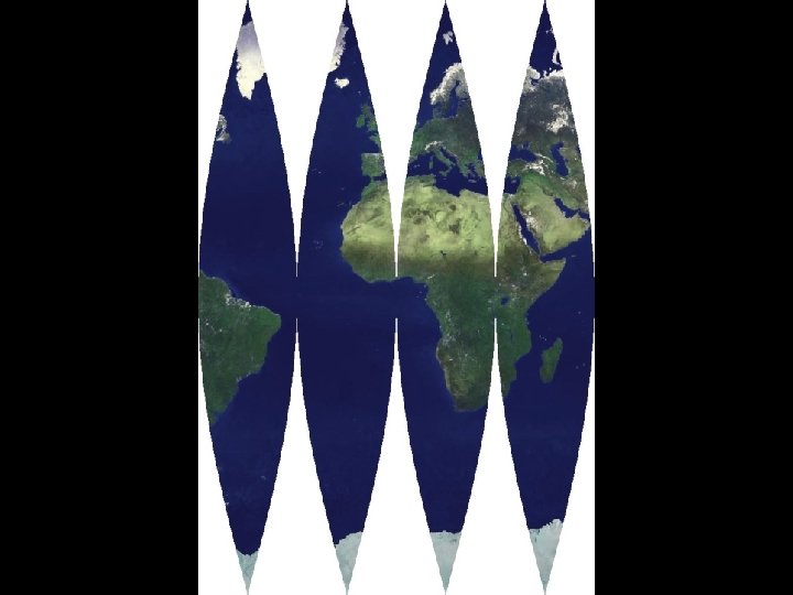
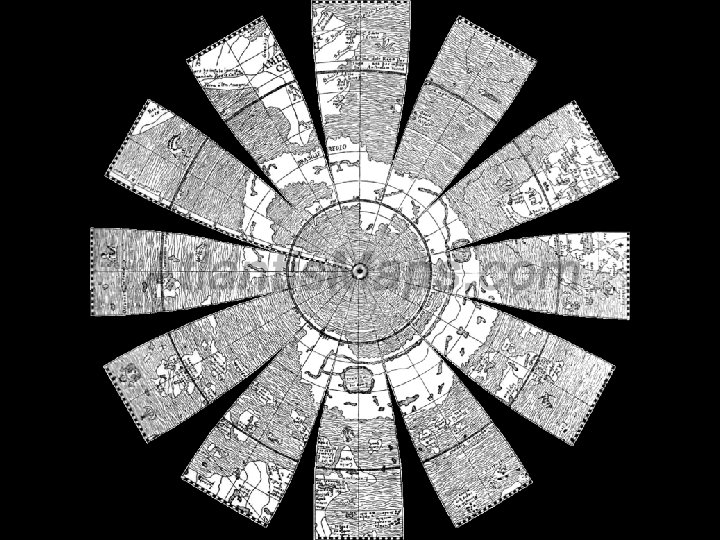
A map projection is a method for mapping spatial patterns on a curved surface (the Earth’s surface) to a flat surface.

nan imaginary light is “projected” onto a “developable surface” na variety of different projection models exist

cone as developable surface secant cone tangent cone

cylinder as developable surface tangent cylinders

plane as developable surface

Map projections always introduce error and distortion

Map projections always introduce error and distortion

Map projections always introduce error and distortion

Map projections always introduce error and distortion Distortion may be minimized in one or more of the following properties: o o Shape … conformal Distance … equidistant Direction … true direction Area … equal area

Exactly what are map projections? Sets of mathematical equations that convert coordinates from one system to another input unprojected angles (lat/long) output projected Cartesian coordinates

How do projections work on a programmatic level? o o o each set of "coordinates" is transformed using a specific projection equation from one system to another angular measurements can be converted to Cartesian coordinates one set of Cartesian coordinates can be converted to a different measurement framework Projection, zone, datum (units) X Y geographic, NAD 27 (decimal degrees) -122. 35° 47. 62° UTM, Zone 10, NAD 27 (meters) 548843. 5049 5274052. 0957 State Plane, WA-N, NAD 83 (feet) 1266092. 5471 229783. 3093

How does Arc. GIS handle map projections in data frames? o o Project data frames to see or measure features under different projection parameters Applying a projection on a data frame projects data “on the fly. ” Arc. GIS’s data frame projection equations can handle any input projection. However, sometimes on-the-fly projected data do not properly overlap.

Applying a projection to a data frame is like putting on a pair of glasses You see the map differently, but the data have not changed

How does Arc. GIS handle map projections for data? n Projecting data creates a new data set on the file system n Data can be projected so that incompatibly projected data sets can be made to match. n Arc. GIS’s projection engine can go in and out of a large number of different projections, coordinate systems, and datums.

Geographic “projection”

Examples of different projections n Shape Area Direction Distance Albers (Conic) Shape along the standard parallels is accurate and minimally distorted in the region between the standard parallels and those regions just beyond. The 90 -degree angles between meridians and parallels are preserved, but because the scale along the lines of longitude does not match the scale along lines of latitude, the final projection is not conformal. All areas are proportional to the same areas on the Earth. Locally true along the standard parallels. Distances are best in the middle latitudes. Along parallels, scale is reduced between the standard parallels and increased beyond them. Along meridians, scale follows an opposite pattern.

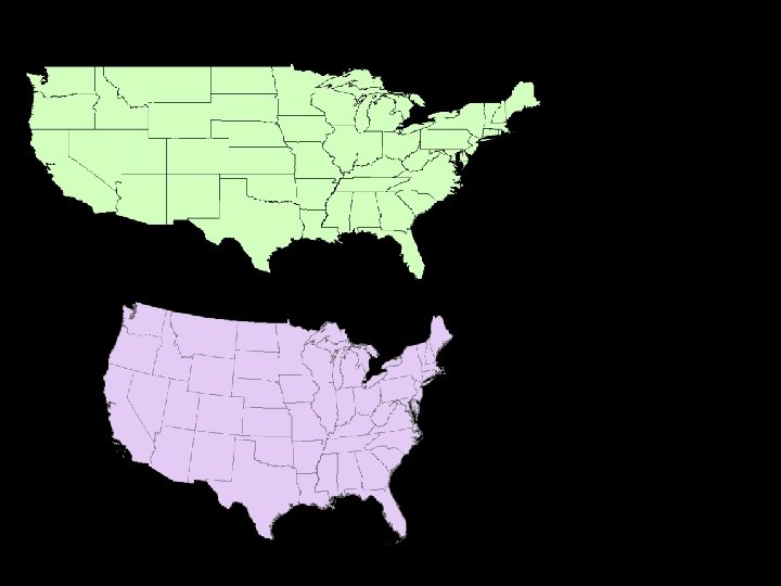
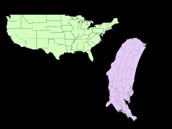
Examples of different projections n Shape Area Direction Distance Lambert Azimuthal Equal Area (Planar) Shape is true along the standard parallels of the normal aspect (Type 1), or the standard lines of the transverse and oblique aspects (Types 2 and 3). Distortion is severe near the poles of the normal aspect or 90° from the central line in the transverse and oblique aspects. There is no area distortion on any of the projections. Local angles are correct along standard parallels or standard lines. Direction is distorted elsewhere. Scale is true along the Equator (Type 1), or the standard lines of the transverse and oblique aspects (Types 2 and 3). Scale distortion is severe near the poles of the normal aspect or 90° from the central line in the transverse and oblique aspects.

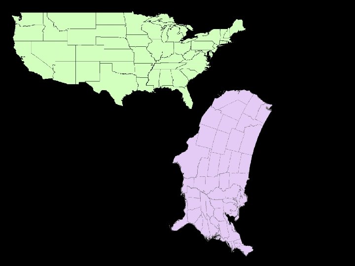
Examples of different projections n Mercator (Cylindrical) Shape Area Direction Distance Conformal. Small shapes are well represented because this projection maintains the local angular relationships. Increasingly distorted toward the polar regions. For example, in the Mercator projection, although Greenland is only one-eighth the size of South America, Greenland appears to be larger. Any straight line drawn on this projection represents an actual compass bearing. These true direction lines are rhumb lines, and generally do not describe the shortest distance between points. Scale is true along the Equator, or along the secant latitudes.

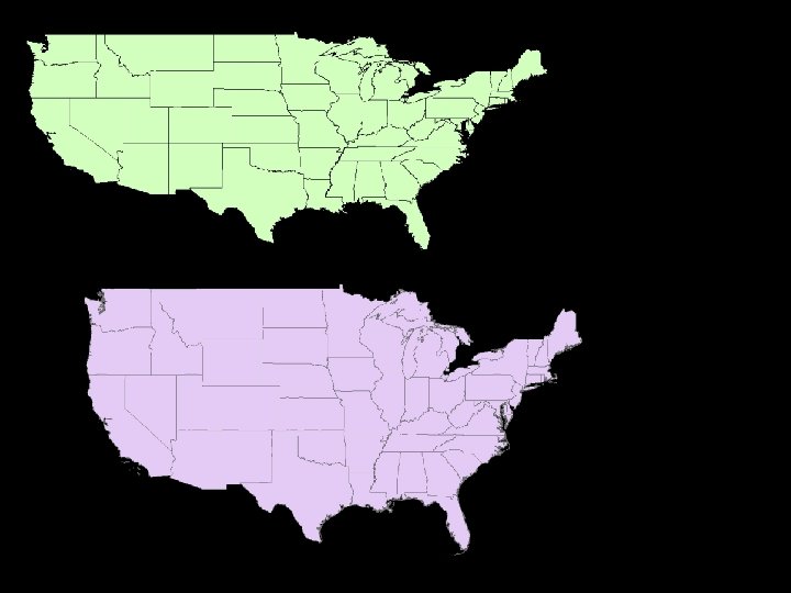
Examples of different projections n Miller (Cylindrical) Shape Area Direction Distance Minimally distorted between 45 th parallels, increasingly toward the poles. Land masses are stretched more east to west than they are north to south. Distortion increases from the Equator toward the poles. Local angles are correct only along the Equator. Correct distance is measured along the Equator.

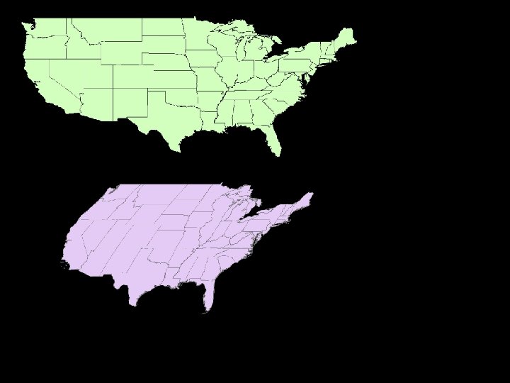
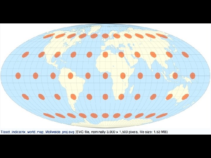
Examples of different projections n Shape Area Direction Distance Mollweide (Pseudocylindrical) Shape is not distorted at the intersection of the central meridian and latitudes 40° 44' N and S. Distortion increases outward from these points and becomes severe at the edges of the projection. Equal-area. Local angles are true only at the intersection of the central meridian and latitudes 40° 44' N and S. Direction is distorted elsewhere. Scale is true along latitudes 40° 44' N and S. Distortion increases with distance from these lines and becomes severe at the edges of the projection.

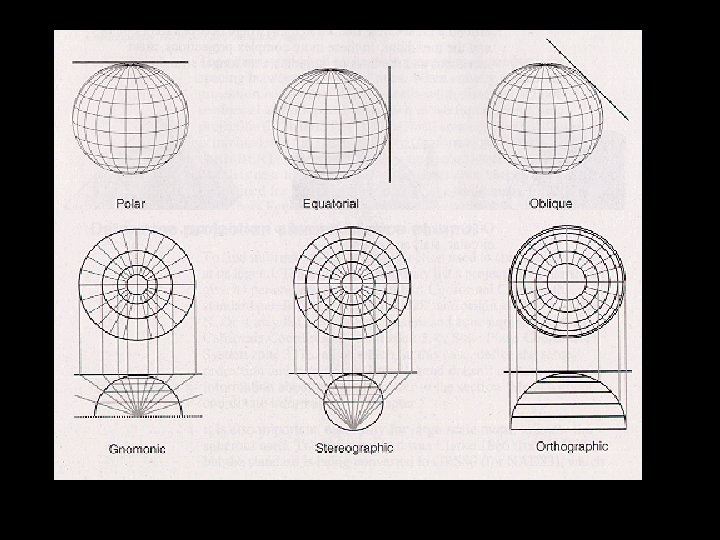
Examples of different projections n Shape Area Direction Distance Orthographic Minimal distortion near the center; maximal distortion near the edge. The areal scale decreases with distance from the center. Areal scale is zero at the edge of the hemisphere. True direction from the central point. The radial scale decreases with distance from the center and becomes zero on the edges. The scale perpendicular to the radii, along the parallels of the polar aspect, is accurate.

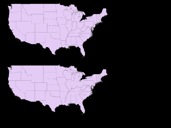
Examples of different projections n Shape Area Direction Distance Robinson (Pseudocylindrical) Shape distortion is very low within 45° of the origin and along the Equator. Distortion is very low within 45° of the origin and along the Equator. Generally distorted. Generally, scale is made true along latitudes 38° N and S. Scale is constant along any given latitude, and for the latitude of opposite sign.

Coordinate Systems

Coordinates n Features on spherical surfaces are not easy to measure n Features on planes are easy to measure and calculate n n n distance angle area n Coordinate systems provide a measurement framework

Coordinates n. Lat/long system measures angles on spherical surfaces n 60º east of PM n 55º north of equator

Lat/long values are NOT Cartesian (X, Y) coordinates constant angular deviations do not have constant distance deviations 1° of longitude at the equator 1° of longitude near the poles

GIS software uses planar measurements on Cartesian planes

Coordinate systems

Coordinate systems Examples of different coordinate/projection systems n State Plane n Universal Transverse Mercator (UTM)

Coordinate systems State Plane Codified in 1930 s n Use of numeric zones for shorthand n SPCS (State Plane Coordinate System) n FIPS (Federal Information Processing System) n n Uses one or more of 3 different projections: Lambert Conformal Conic (east-west orientation ) n Transverse Mercator (north-south orientation) n Oblique Mercator (nw-se or ne-sw orientation) n

Coordinate systems Universal Transverse Mercator (UTM) n Based on the Transverse Mercator projection n 60 zones (each 6° wide) n false n Y-0 eastings set at south pole or equator

Universal Transverse Mercator (UTM) Washington state is in Zones 10 & 11

Coordinate systems Every place on earth falls in a particular zone

Datums

Datums A system that allows us to place a coordinate system on the earth’s surface Initial point Secondary point Model of the earth Known geoidal separation at the initial point

Datums Commonly used datums in North American Datum of 1927 (NAD 27) n NAD 83 n World Geodetic System of 1984 (WGS 84) n

Projecting spatial data sets Used for going between projections Source data sources may not be compatible UTM 36 UTM 34 Lake Victoria is not in central Africa

Projecting spatial data sets n Used for going between projections • Data sets are now compatible both are now UTM 34 Lake Victoria really is in east Africa