Production Function l The firms production function for

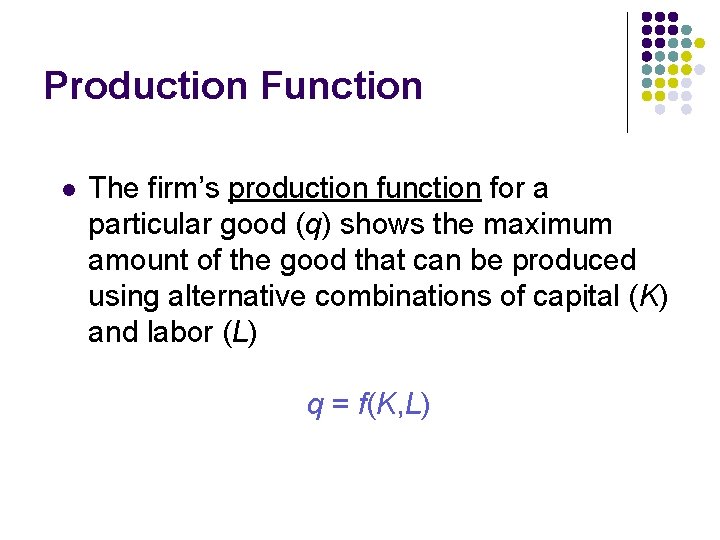
Production Function l The firm’s production function for a particular good (q) shows the maximum amount of the good that can be produced using alternative combinations of capital (K) and labor (L) q = f(K, L)

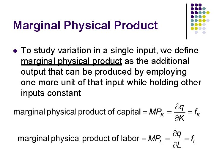
Marginal Physical Product l To study variation in a single input, we define marginal physical product as the additional output that can be produced by employing one more unit of that input while holding other inputs constant

Diminishing Marginal Productivity l l Because of diminishing marginal productivity, 19 th century economist Thomas Malthus worried about the effect of population growth on labor productivity But changes in the marginal productivity of labor over time also depend on changes in other inputs such as capital

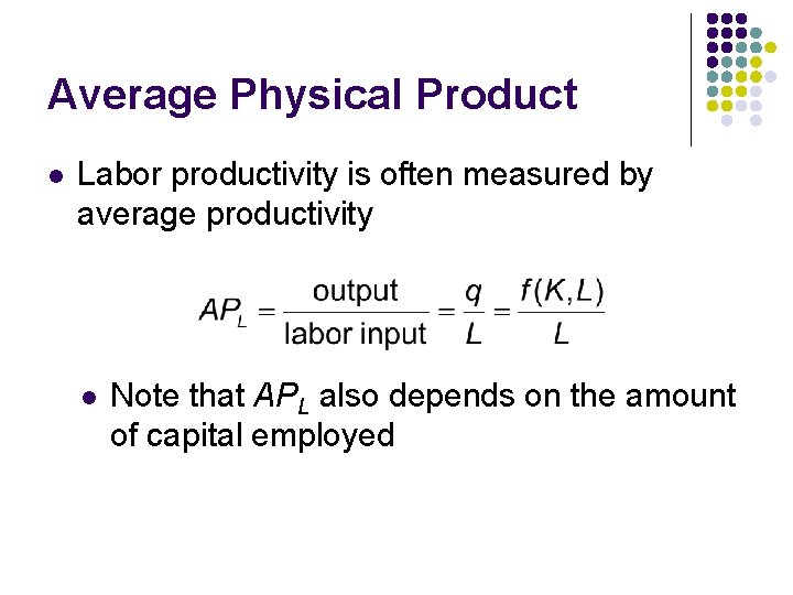
Average Physical Product l Labor productivity is often measured by average productivity l Note that APL also depends on the amount of capital employed

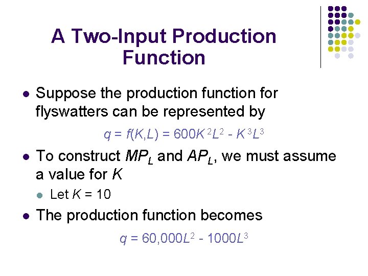
A Two-Input Production Function l Suppose the production function for flyswatters can be represented by q = f(K, L) = 600 K 2 L 2 - K 3 L 3 l To construct MPL and APL, we must assume a value for K l l Let K = 10 The production function becomes q = 60, 000 L 2 - 1000 L 3

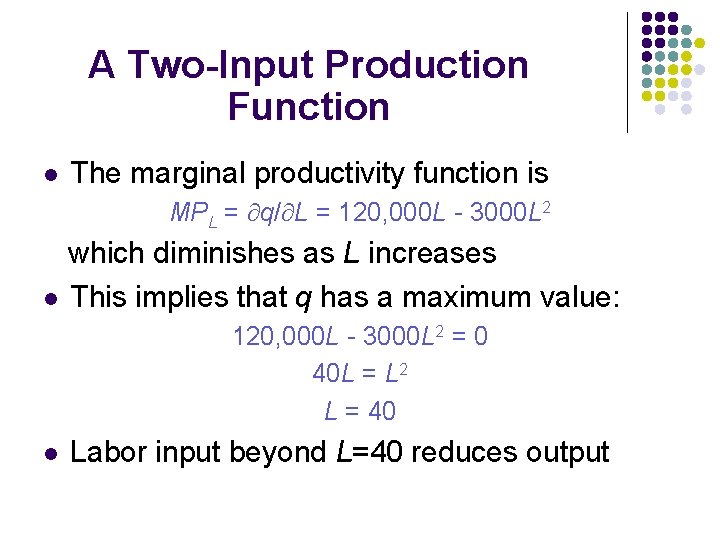
A Two-Input Production Function l The marginal productivity function is MPL = q/ L = 120, 000 L - 3000 L 2 which diminishes as L increases l This implies that q has a maximum value: 120, 000 L - 3000 L 2 = 0 40 L = L 2 L = 40 l Labor input beyond L=40 reduces output

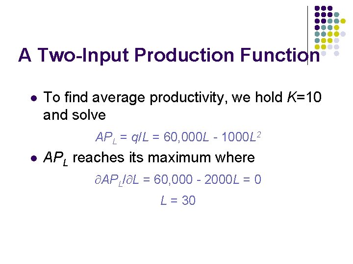
A Two-Input Production Function l To find average productivity, we hold K=10 and solve APL = q/L = 60, 000 L - 1000 L 2 l APL reaches its maximum where APL/ L = 60, 000 - 2000 L = 0 L = 30

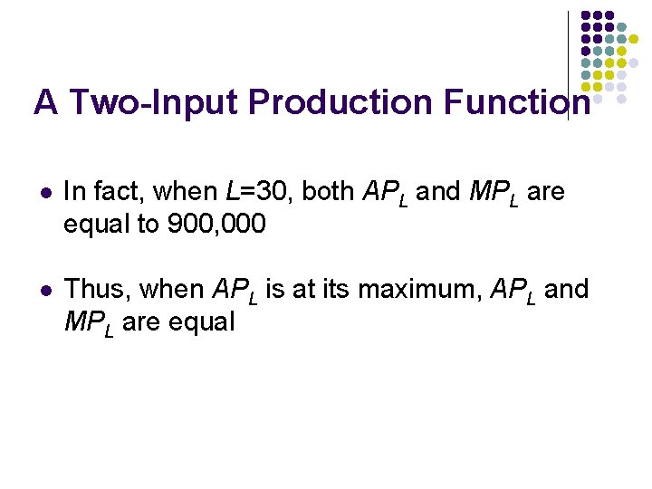
A Two-Input Production Function l In fact, when L=30, both APL and MPL are equal to 900, 000 l Thus, when APL is at its maximum, APL and MPL are equal

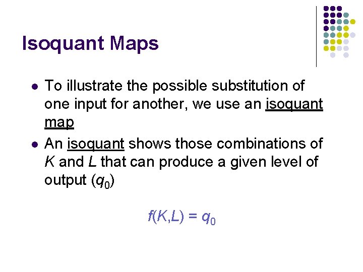
Isoquant Maps l l To illustrate the possible substitution of one input for another, we use an isoquant map An isoquant shows those combinations of K and L that can produce a given level of output (q 0) f(K, L) = q 0

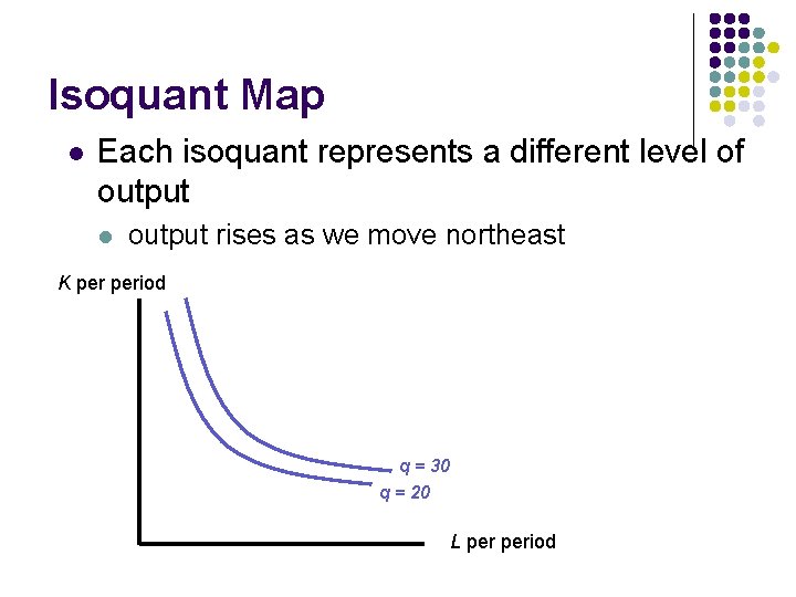
Isoquant Map l Each isoquant represents a different level of output l output rises as we move northeast K period q = 30 q = 20 L period

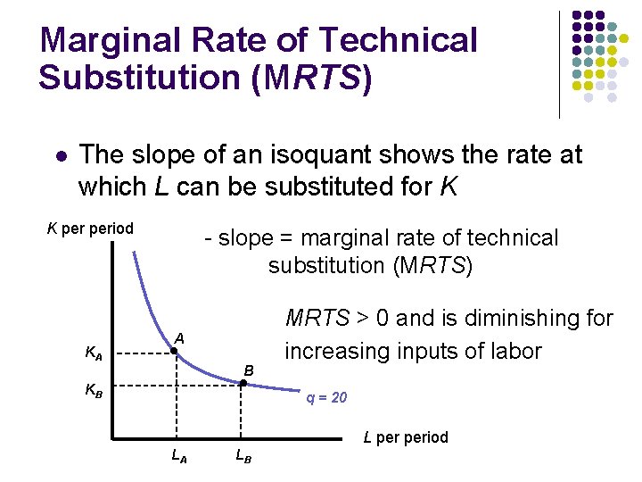
Marginal Rate of Technical Substitution (MRTS) l The slope of an isoquant shows the rate at which L can be substituted for K K period KA - slope = marginal rate of technical substitution (MRTS) A B KB MRTS > 0 and is diminishing for increasing inputs of labor q = 20 L period LA LB

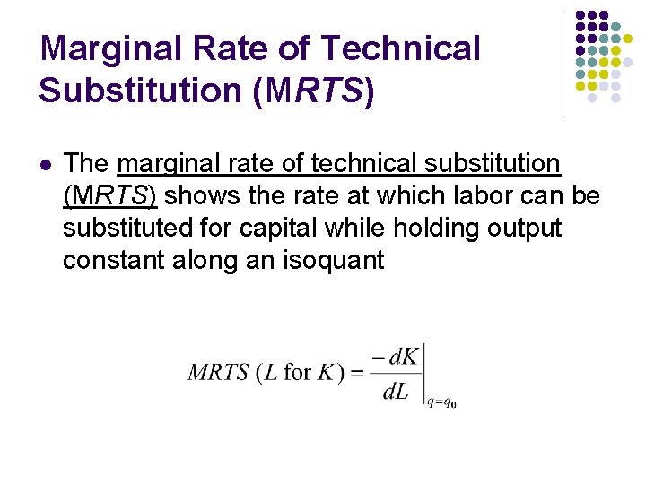
Marginal Rate of Technical Substitution (MRTS) l The marginal rate of technical substitution (MRTS) shows the rate at which labor can be substituted for capital while holding output constant along an isoquant

Returns to Scale l l l How does output respond to increases in all inputs together? Suppose that all inputs are doubled, would output double? Returns to scale have been of interest to economists since the days of Adam Smith

Returns to Scale l Smith identified two forces that come into operation as inputs are doubled l l greater division of labor and specialization of labor loss in efficiency because management may become more difficult given the larger scale of the firm

Returns to Scale l It is possible for a production function to exhibit constant returns to scale for some levels of input usage and increasing or decreasing returns for other levels l economists refer to the degree of returns to scale with the implicit notion that only a fairly narrow range of variation in input usage and the related level of output is being considered

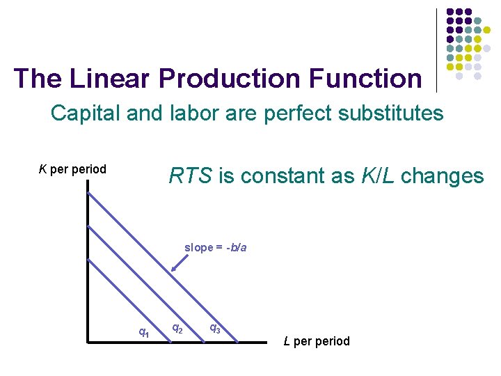
The Linear Production Function Capital and labor are perfect substitutes K period RTS is constant as K/L changes slope = -b/a q 1 q 2 q 3 L period

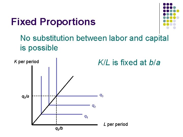
Fixed Proportions No substitution between labor and capital is possible K/L is fixed at b/a K period q 3/a q 2 q 1 q 3/b L period

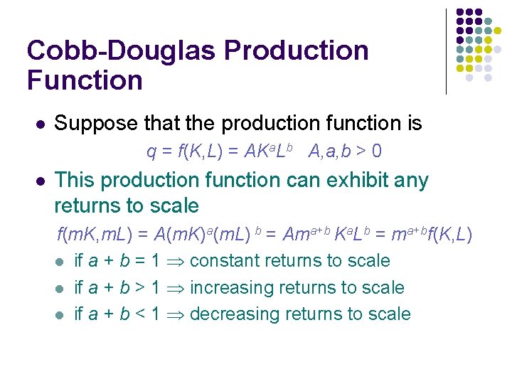
Cobb-Douglas Production Function l Suppose that the production function is q = f(K, L) = AKa. Lb A, a, b > 0 l This production function can exhibit any returns to scale f(m. K, m. L) = A(m. K)a(m. L) b = Ama+b Ka. Lb = ma+bf(K, L) l if a + b = 1 constant returns to scale l if a + b > 1 increasing returns to scale l if a + b < 1 decreasing returns to scale

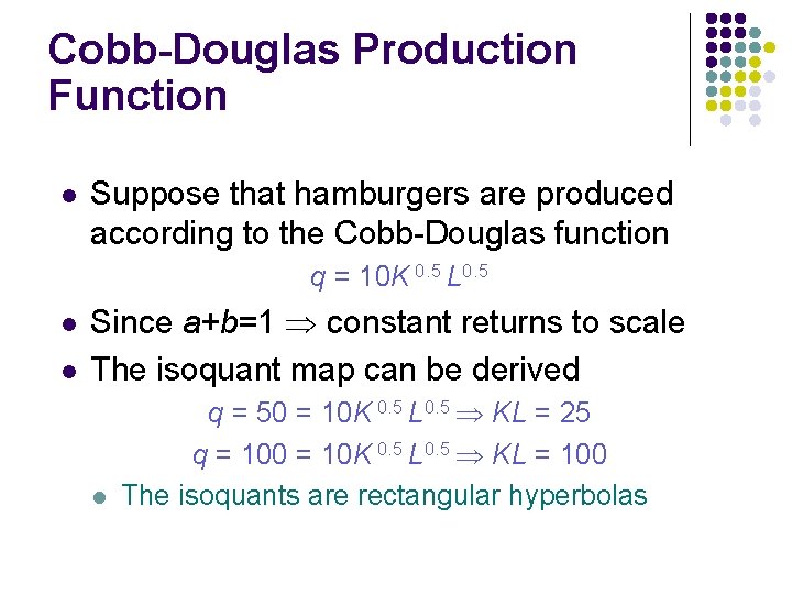
Cobb-Douglas Production Function l Suppose that hamburgers are produced according to the Cobb-Douglas function q = 10 K 0. 5 L 0. 5 l l Since a+b=1 constant returns to scale The isoquant map can be derived l q = 50 = 10 K 0. 5 L 0. 5 KL = 25 q = 100 = 10 K 0. 5 L 0. 5 KL = 100 The isoquants are rectangular hyperbolas

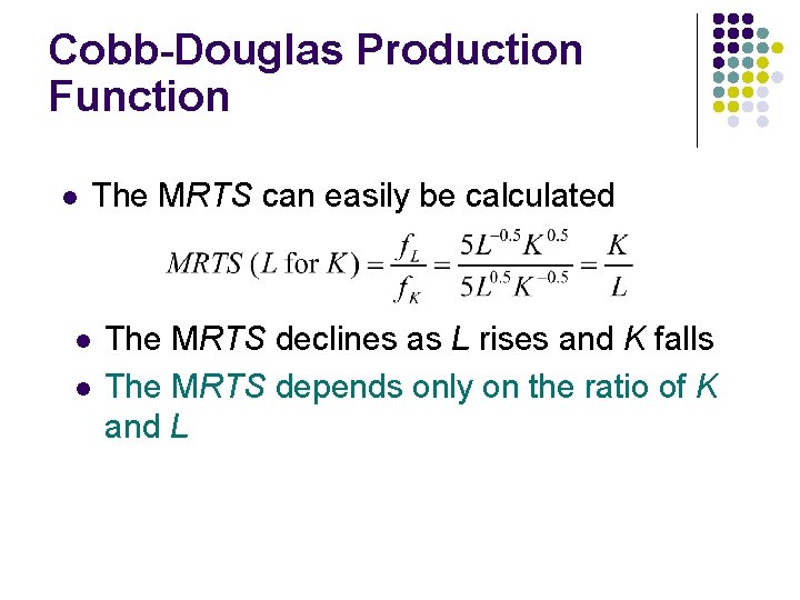
Cobb-Douglas Production Function l The MRTS can easily be calculated l l The MRTS declines as L rises and K falls The MRTS depends only on the ratio of K and L

Technical Progress l l Methods of production change over time Following the development of superior production techniques, the same level of output can be produced with fewer inputs l the isoquant shifts in