Production Functions nvmrao Production Function The firms production


![Technical Progress • For any variable x, [(dx/dt)/x] is the proportional growth rate in Technical Progress • For any variable x, [(dx/dt)/x] is the proportional growth rate in](https://slidetodoc.com/presentation_image/4a1d432591116b1d5d8ab2b32682fa8a/image-65.jpg)
- Slides: 75

Production Functions nvmrao

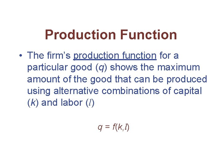
Production Function • The firm’s production function for a particular good (q) shows the maximum amount of the good that can be produced using alternative combinations of capital (k) and labor (l) q = f(k, l)

Short Run & Long Run

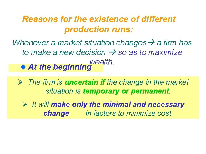
Reasons for the existence of different production runs: Whenever a market situation changes a firm has to make a new decision so as to maximize wealth. At the beginning Ø The firm is uncertain if the change in the market situation is temporary or permanent. Ø It will make only the minimal and necessary change in factors to minimize cost.

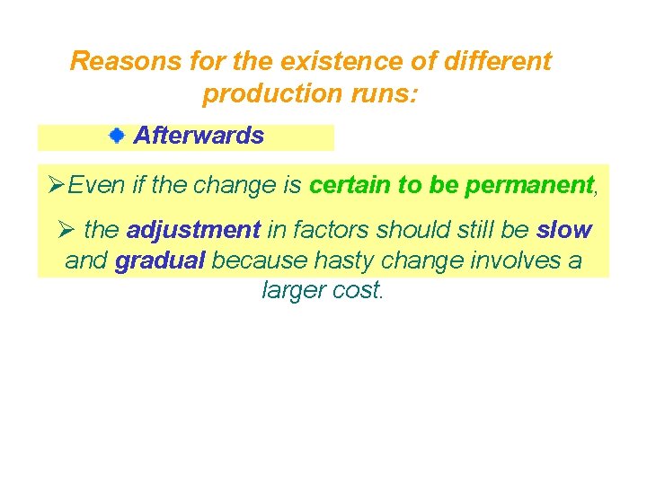
Reasons for the existence of different production runs: Afterwards ØEven if the change is certain to be permanent, Ø the adjustment in factors should still be slow and gradual because hasty change involves a larger cost.

Reasons for the existence of different production runs: Since adjustment is gradual, according to the completeness in the adjustment in factors, three different production runs are classified.

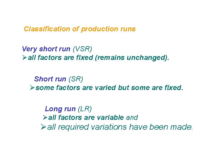
Classification of production runs Very short run (VSR) Øall factors are fixed (remains unchanged). Short run (SR) Øsome factors are varied but some are fixed. Long run (LR) Øall factors are variable and Øall required variations have been made.

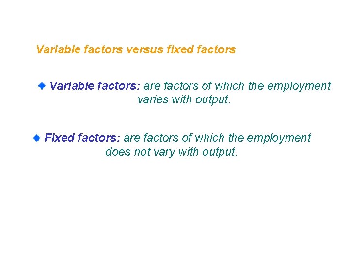
Variable factors versus fixed factors Variable factors: are factors of which the employment varies with output. Fixed factors: are factors of which the employment does not vary with output.

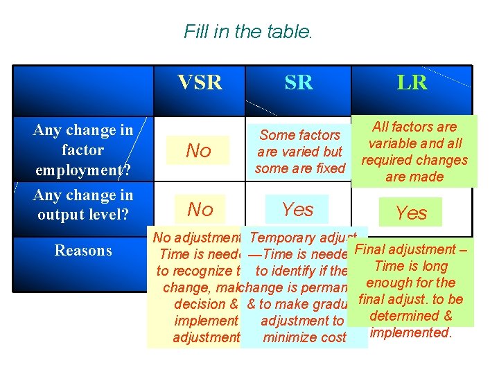
Fill in the table. VSR SR LR Any change in factor employment? No Some factors are varied but some are fixed All factors are variable and all required changes are made Any change in output level? No Yes Reasons No adjustment — Temporary adjust. Time is needed—Time is needed. Final adjustment – Time is long to recognize theto identify if the change, make change is permanentenough for the decision & & to make gradualfinal adjust. to be determined & implement adjustment to implemented. adjustment minimize cost

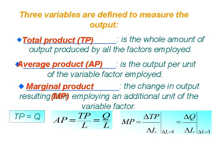
Three variables are defined to measure the output: __________: is the whole amount of Total product (TP) output produced by all the factors employed. Average product (AP) __________: is the output per unit of the variable factor employed. __________: the change in output Marginal product resulting(MP) from employing an additional unit of the variable factor. TP = Q

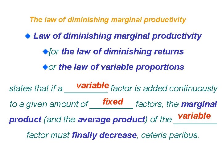
The law of diminishing marginal productivity Law of diminishing marginal productivity [or the law of diminishing returns or the law of variable proportions variable factor is added continuously states that if a _____ fixed to a given amount of _____ factors, the marginal variable product (and the average product) of the _____ factor must finally decrease, ceteris paribus.

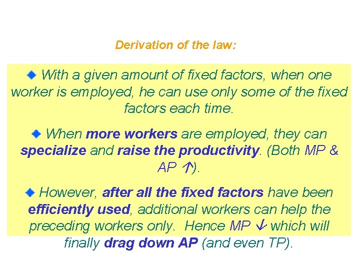
Derivation of the law: With a given amount of fixed factors, when one worker is employed, he can use only some of the fixed factors each time. When more workers are employed, they can specialize and raise the productivity. (Both MP & AP ). However, after all the fixed factors have been efficiently used, additional workers can help the preceding workers only. Hence MP which will finally drag down AP (and even TP).

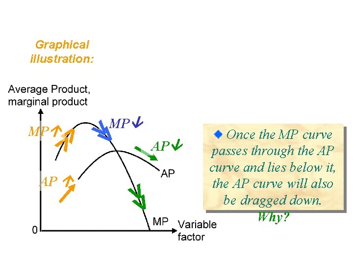
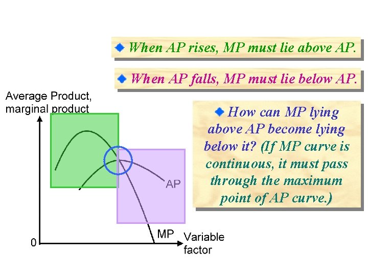
Graphical illustration: >> AP >> MP Once the MP curve passes through the AP curve and lies below it, the AP curve will also be dragged down. Why?

When AP rises, MP must lie above AP. When AP falls, MP must lie below AP. How can MP lying above AP become lying below it? (If MP curve is continuous, it must pass through the maximum point of AP curve. )

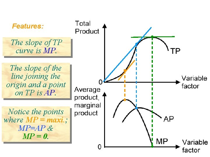
Features: The slope of TP curve is MP. The slope of the line joining the origin and a point on TP is AP. Notice the points where MP = maxi. ; MP=AP & MP = 0.

Implications of the law (if the law is violated) By adding units of fertilizer or worker continuously to a given plot of land, no matter how small its size is, TP can be increased continuously. Enough food can be produced to feed all the people in the world. An infinitesimal piece of land is adequate to supply the amount of food required. Hence the supply of land is no longer scarce. Land price would drop to zero. MP of workers cultivating superior land does not fall and is always larger than MP of workers cultivating inferior land. No inferior land would be cultivated.

Implications of the law (if the law holds) If the amount of land is fixed, TP cannot be increased significantly (∵ MP & AP ) to feed all the people in the world. Hence to raise production, more land is needed. However, as the supply of land is limited and scarce, under competition, land price must be positive. Once MP of superior land falls below MP of inferior land, inferior land will also be cultivated.

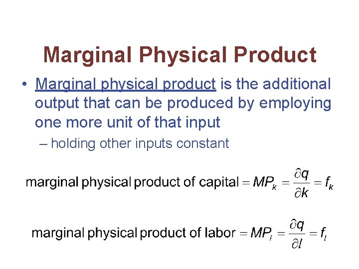
Marginal Physical Product • Marginal physical product is the additional output that can be produced by employing one more unit of that input – holding other inputs constant

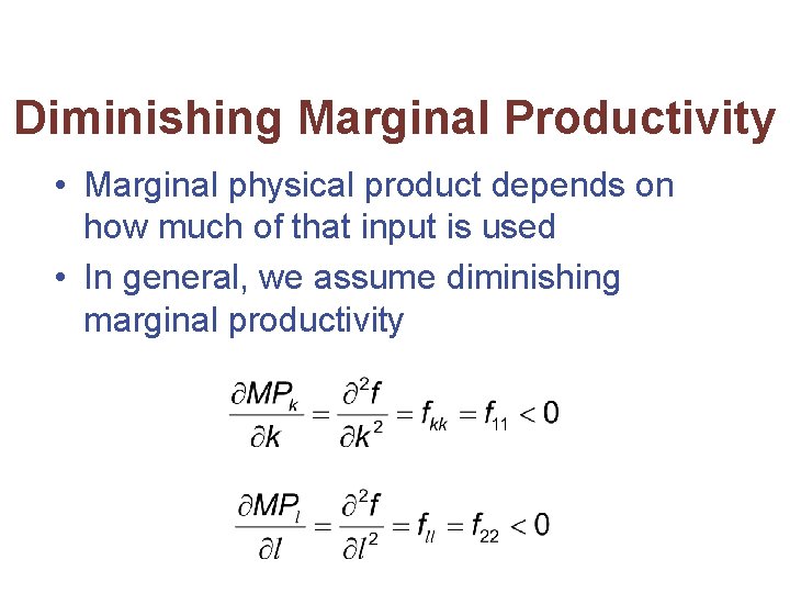
Diminishing Marginal Productivity • Marginal physical product depends on how much of that input is used • In general, we assume diminishing marginal productivity

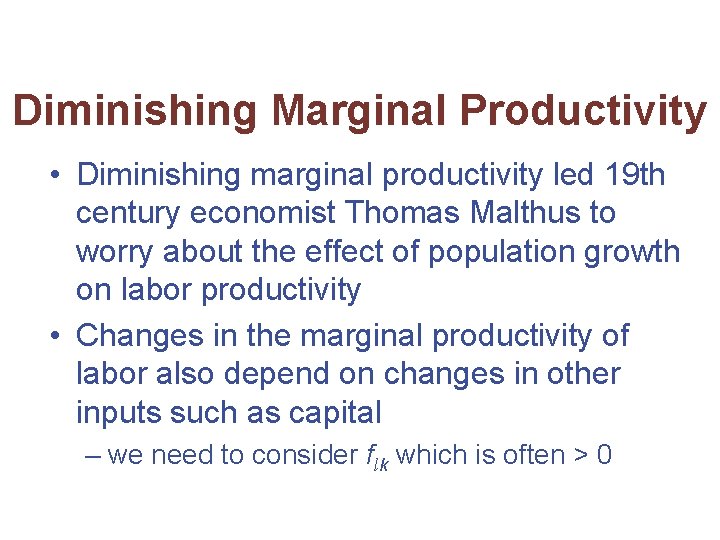
Diminishing Marginal Productivity • Diminishing marginal productivity led 19 th century economist Thomas Malthus to worry about the effect of population growth on labor productivity • Changes in the marginal productivity of labor also depend on changes in other inputs such as capital – we need to consider flk which is often > 0

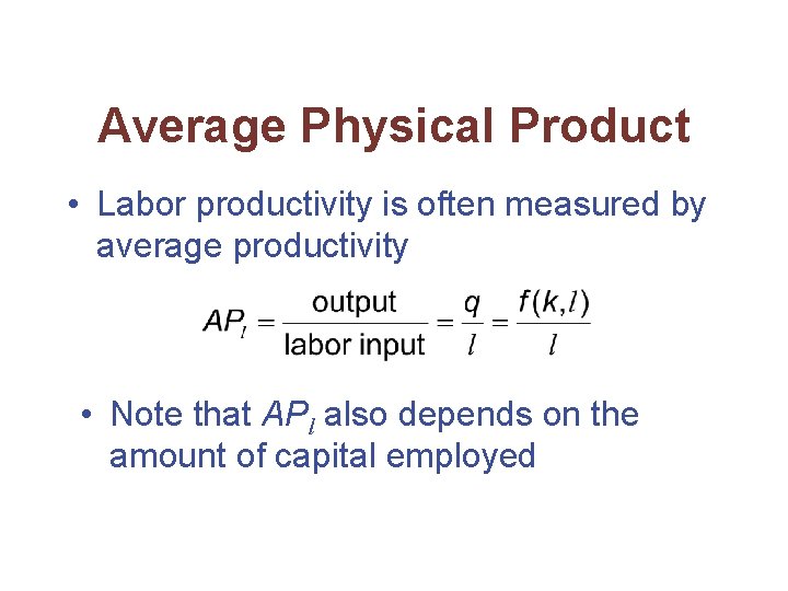
Average Physical Product • Labor productivity is often measured by average productivity • Note that APl also depends on the amount of capital employed

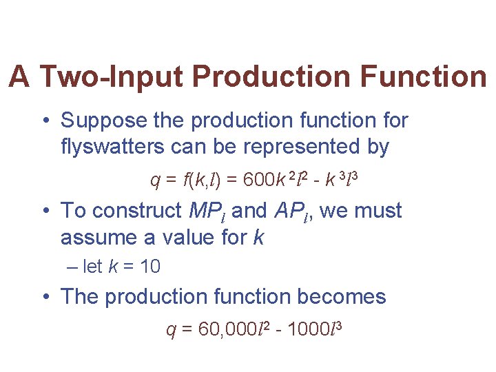
A Two-Input Production Function • Suppose the production function for flyswatters can be represented by q = f(k, l) = 600 k 2 l 2 - k 3 l 3 • To construct MPl and APl, we must assume a value for k – let k = 10 • The production function becomes q = 60, 000 l 2 - 1000 l 3

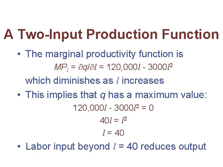
A Two-Input Production Function • The marginal productivity function is MPl = q/ l = 120, 000 l - 3000 l 2 which diminishes as l increases • This implies that q has a maximum value: 120, 000 l - 3000 l 2 = 0 40 l = l 2 l = 40 • Labor input beyond l = 40 reduces output

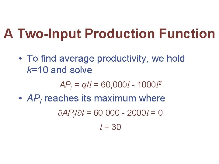
A Two-Input Production Function • To find average productivity, we hold k=10 and solve APl = q/l = 60, 000 l - 1000 l 2 • APl reaches its maximum where APl/ l = 60, 000 - 2000 l = 0 l = 30

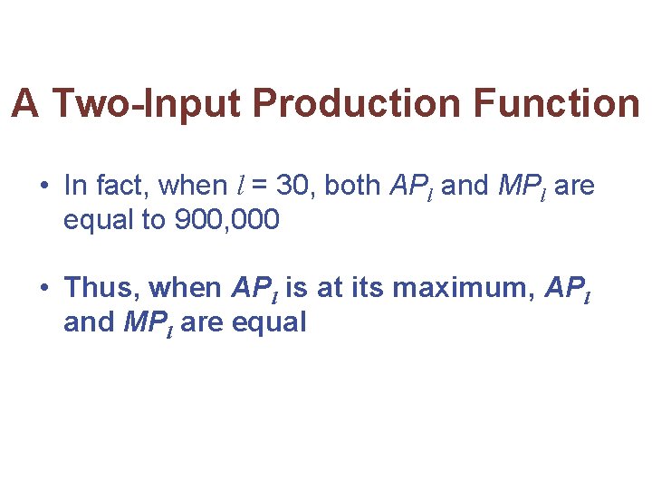
A Two-Input Production Function • In fact, when l = 30, both APl and MPl are equal to 900, 000 • Thus, when APl is at its maximum, APl and MPl are equal

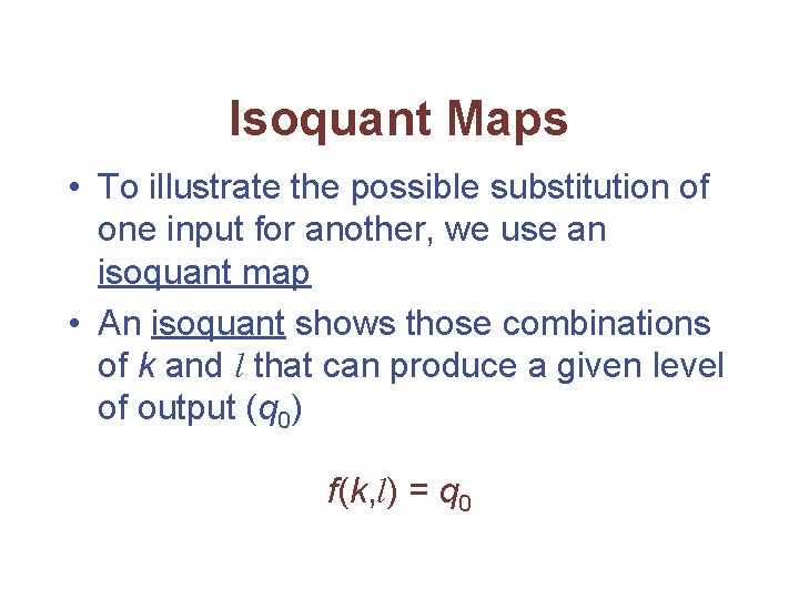
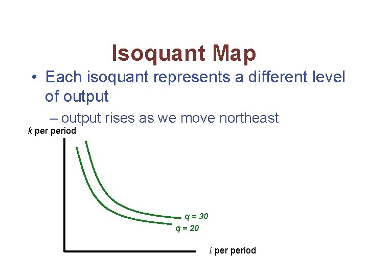
Isoquant Maps • To illustrate the possible substitution of one input for another, we use an isoquant map • An isoquant shows those combinations of k and l that can produce a given level of output (q 0) f(k, l) = q 0

Isoquant Map • Each isoquant represents a different level of output – output rises as we move northeast k period q = 30 q = 20 l period

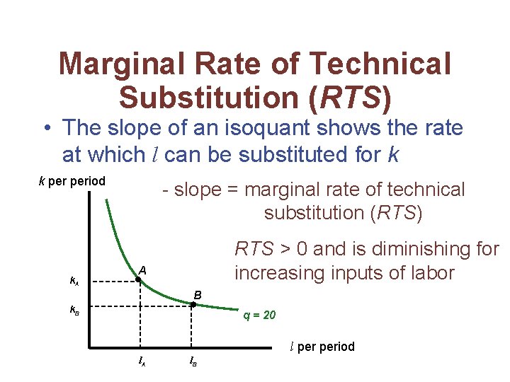
Marginal Rate of Technical Substitution (RTS) • The slope of an isoquant shows the rate at which l can be substituted for k k period k. A - slope = marginal rate of technical substitution (RTS) RTS > 0 and is diminishing for increasing inputs of labor A B k. B q = 20 l period l. A l. B

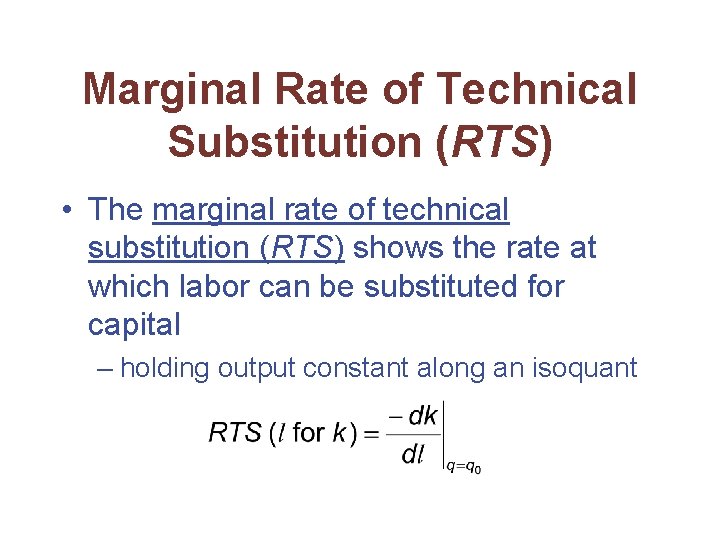
Marginal Rate of Technical Substitution (RTS) • The marginal rate of technical substitution (RTS) shows the rate at which labor can be substituted for capital – holding output constant along an isoquant

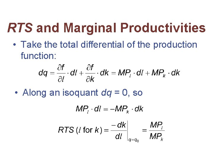
RTS and Marginal Productivities • Take the total differential of the production function: • Along an isoquant dq = 0, so

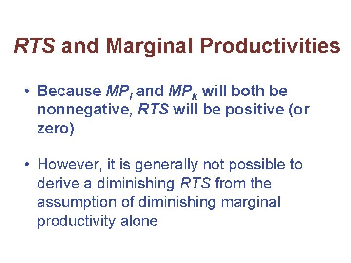
RTS and Marginal Productivities • Because MPl and MPk will both be nonnegative, RTS will be positive (or zero) • However, it is generally not possible to derive a diminishing RTS from the assumption of diminishing marginal productivity alone

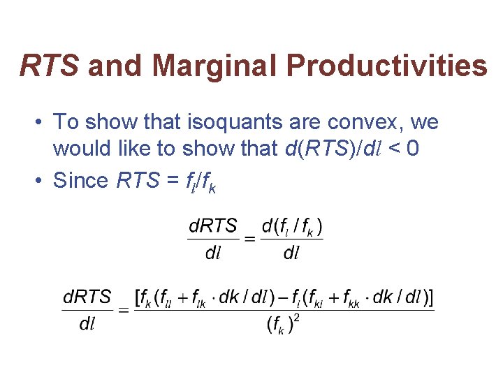
RTS and Marginal Productivities • To show that isoquants are convex, we would like to show that d(RTS)/dl < 0 • Since RTS = fl/fk

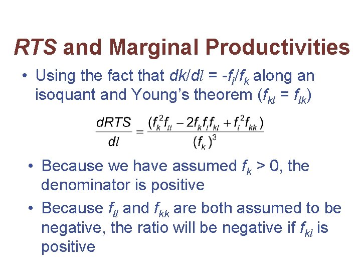
RTS and Marginal Productivities • Using the fact that dk/dl = -fl/fk along an isoquant and Young’s theorem (fkl = flk) • Because we have assumed fk > 0, the denominator is positive • Because fll and fkk are both assumed to be negative, the ratio will be negative if fkl is positive

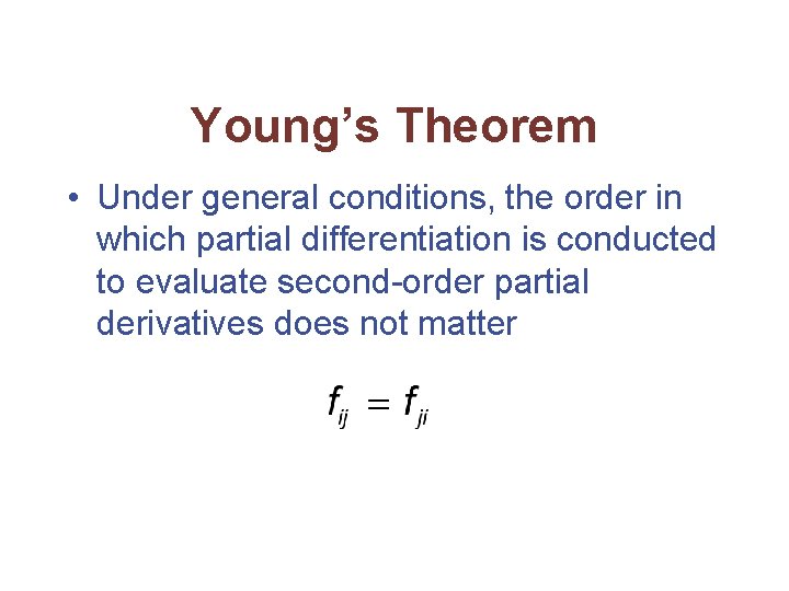
Young’s Theorem • Under general conditions, the order in which partial differentiation is conducted to evaluate second-order partial derivatives does not matter

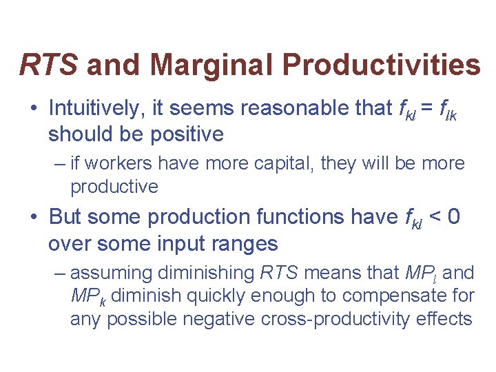
RTS and Marginal Productivities • Intuitively, it seems reasonable that fkl = flk should be positive – if workers have more capital, they will be more productive • But some production functions have fkl < 0 over some input ranges – assuming diminishing RTS means that MPl and MPk diminish quickly enough to compensate for any possible negative cross-productivity effects

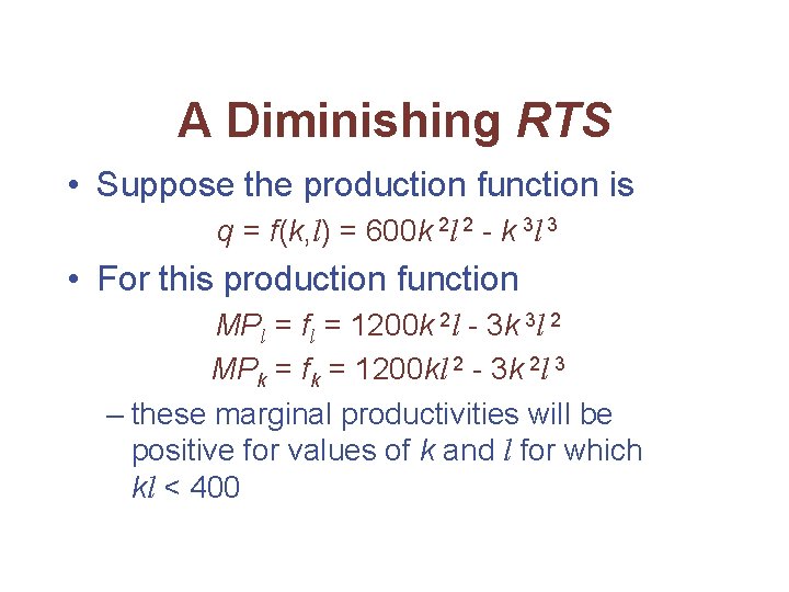
A Diminishing RTS • Suppose the production function is q = f(k, l) = 600 k 2 l 2 - k 3 l 3 • For this production function MPl = fl = 1200 k 2 l - 3 k 3 l 2 MPk = fk = 1200 kl 2 - 3 k 2 l 3 – these marginal productivities will be positive for values of k and l for which kl < 400

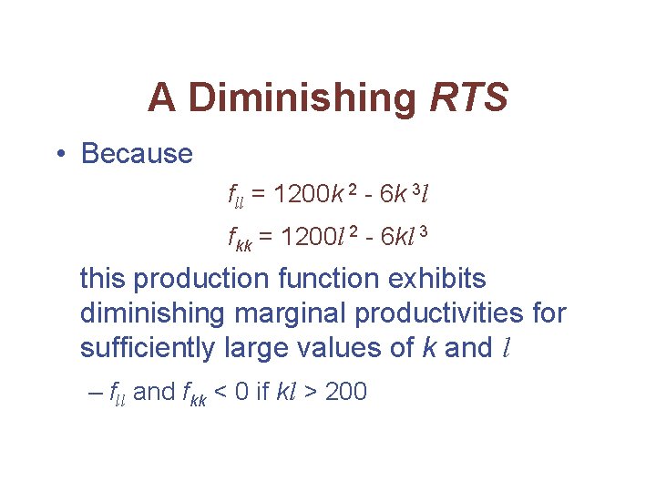
A Diminishing RTS • Because fll = 1200 k 2 - 6 k 3 l fkk = 1200 l 2 - 6 kl 3 this production function exhibits diminishing marginal productivities for sufficiently large values of k and l – fll and fkk < 0 if kl > 200

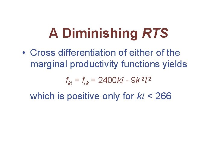
A Diminishing RTS • Cross differentiation of either of the marginal productivity functions yields fkl = flk = 2400 kl - 9 k 2 l 2 which is positive only for kl < 266

Returns to Scale • How does output respond to increases in all inputs together? – suppose that all inputs are doubled, would output double? • Returns to scale have been of interest to economists since the days of Adam Smith

Returns to Scale • Two forces that occur as inputs are doubled – greater division of labor and specialization of function – loss in efficiency • management may become more difficult

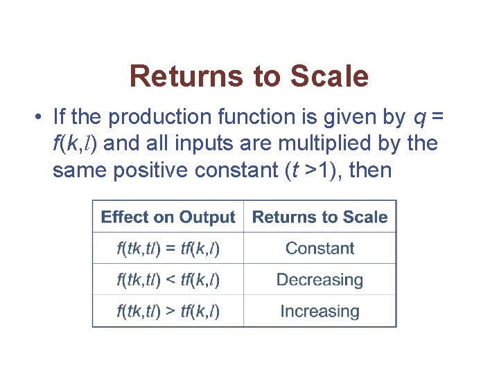
Returns to Scale • If the production function is given by q = f(k, l) and all inputs are multiplied by the same positive constant (t >1), then

Returns to Scale • It is possible for a production function to exhibit constant returns to scale for some levels of input usage and increasing or decreasing returns for other levels – the degree of returns to scale is generally defined within a fairly narrow range of variation in input usage

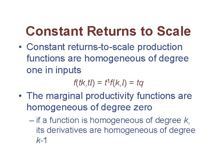
Constant Returns to Scale • Constant returns-to-scale production functions are homogeneous of degree one in inputs f(tk, tl) = t 1 f(k, l) = tq • The marginal productivity functions are homogeneous of degree zero – if a function is homogeneous of degree k, its derivatives are homogeneous of degree k-1

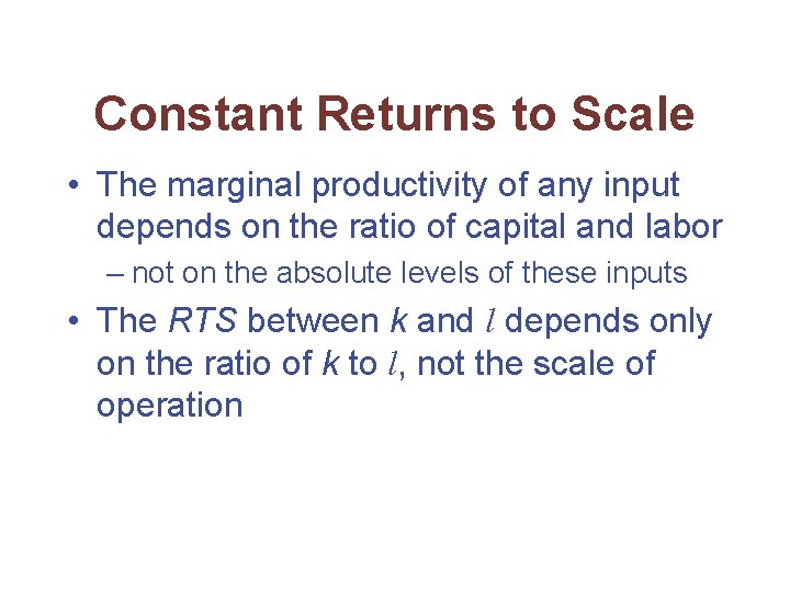
Constant Returns to Scale • The marginal productivity of any input depends on the ratio of capital and labor – not on the absolute levels of these inputs • The RTS between k and l depends only on the ratio of k to l, not the scale of operation

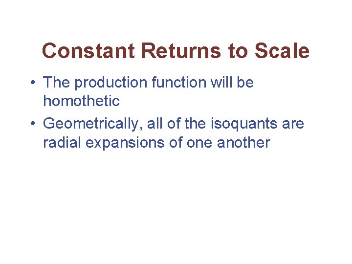
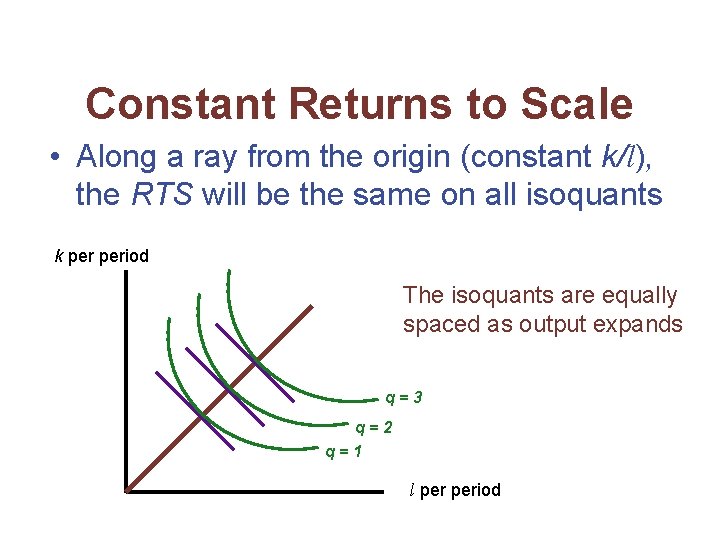
Constant Returns to Scale • The production function will be homothetic • Geometrically, all of the isoquants are radial expansions of one another

Constant Returns to Scale • Along a ray from the origin (constant k/l), the RTS will be the same on all isoquants k period The isoquants are equally spaced as output expands q=3 q=2 q=1 l period

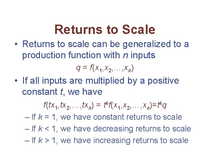
Returns to Scale • Returns to scale can be generalized to a production function with n inputs q = f(x 1, x 2, …, xn) • If all inputs are multiplied by a positive constant t, we have f(tx 1, tx 2, …, txn) = tkf(x 1, x 2, …, xn)=tkq – If k = 1, we have constant returns to scale – If k < 1, we have decreasing returns to scale – If k > 1, we have increasing returns to scale

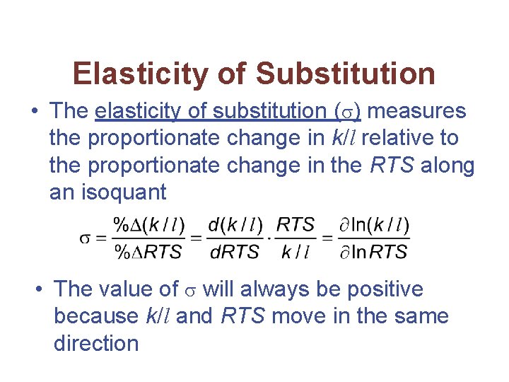
Elasticity of Substitution • The elasticity of substitution ( ) measures the proportionate change in k/l relative to the proportionate change in the RTS along an isoquant • The value of will always be positive because k/l and RTS move in the same direction

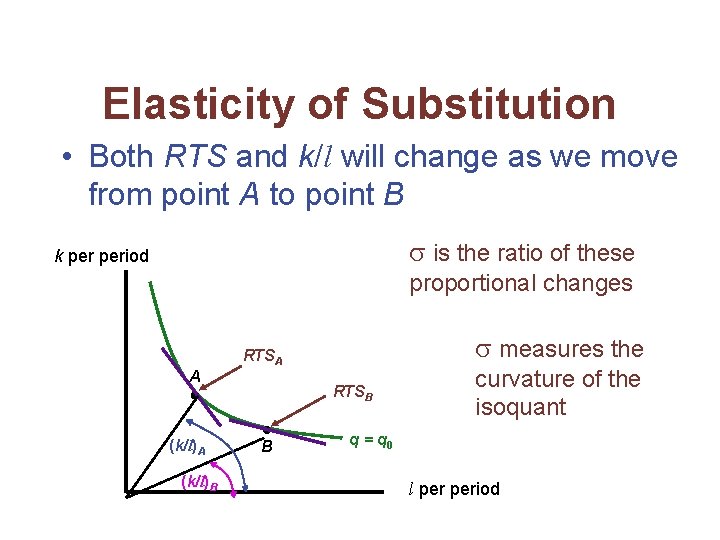
Elasticity of Substitution • Both RTS and k/l will change as we move from point A to point B is the ratio of these k period proportional changes measures the RTSA A (k/l)B RTSB B curvature of the isoquant q = q 0 l period

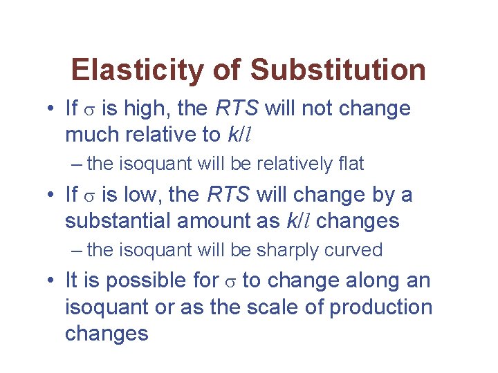
Elasticity of Substitution • If is high, the RTS will not change much relative to k/l – the isoquant will be relatively flat • If is low, the RTS will change by a substantial amount as k/l changes – the isoquant will be sharply curved • It is possible for to change along an isoquant or as the scale of production changes

Elasticity of Substitution • If we define the elasticity of substitution between two inputs to be the proportionate change in the ratio of the two inputs to the proportionate change in RTS, we need to hold output and the levels of other inputs constant

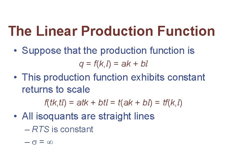
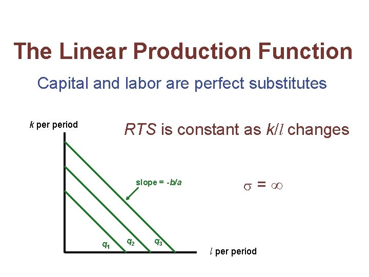
The Linear Production Function • Suppose that the production function is q = f(k, l) = ak + bl • This production function exhibits constant returns to scale f(tk, tl) = atk + btl = t(ak + bl) = tf(k, l) • All isoquants are straight lines – RTS is constant – =

The Linear Production Function Capital and labor are perfect substitutes k period RTS is constant as k/l changes slope = -b/a q 1 q 2 q 3 = l period

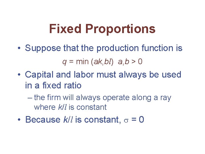
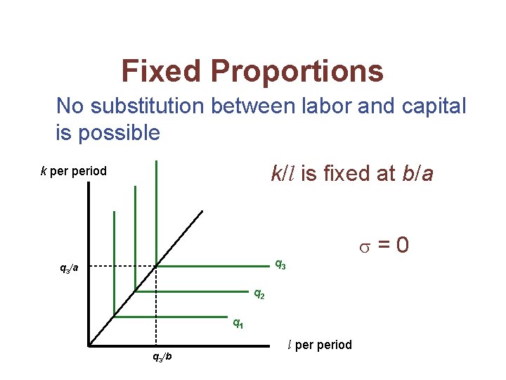
Fixed Proportions • Suppose that the production function is q = min (ak, bl) a, b > 0 • Capital and labor must always be used in a fixed ratio – the firm will always operate along a ray where k/l is constant • Because k/l is constant, = 0

Fixed Proportions No substitution between labor and capital is possible k/l is fixed at b/a k period =0 q 3/a q 2 q 1 q 3/b l period

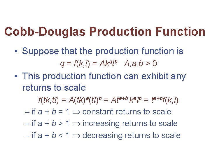
Cobb-Douglas Production Function • Suppose that the production function is q = f(k, l) = Akalb A, a, b > 0 • This production function can exhibit any returns to scale f(tk, tl) = A(tk)a(tl)b = Ata+b kalb = ta+bf(k, l) – if a + b = 1 constant returns to scale – if a + b > 1 increasing returns to scale – if a + b < 1 decreasing returns to scale

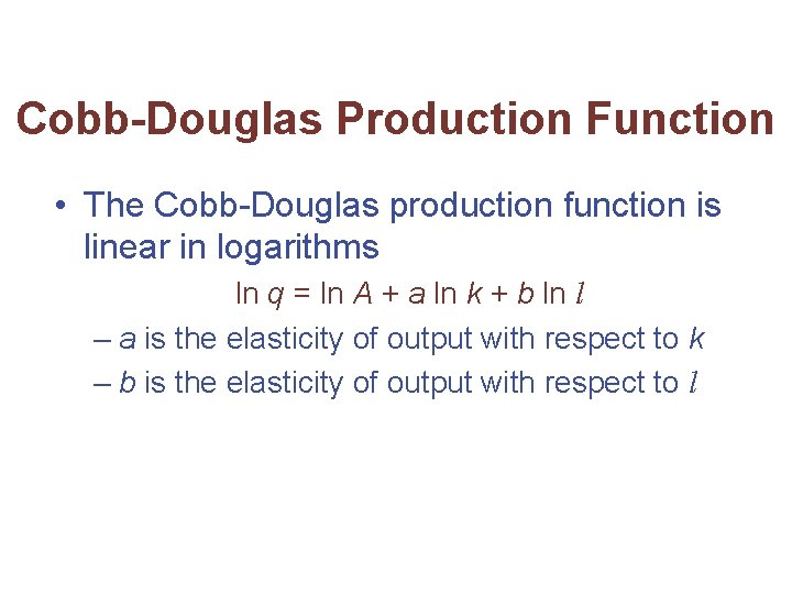
Cobb-Douglas Production Function • The Cobb-Douglas production function is linear in logarithms ln q = ln A + a ln k + b ln l – a is the elasticity of output with respect to k – b is the elasticity of output with respect to l

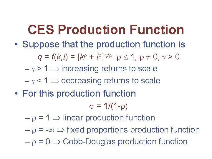
CES Production Function • Suppose that the production function is q = f(k, l) = [k + l ] / 1, 0, > 0 – > 1 increasing returns to scale – < 1 decreasing returns to scale • For this production function = 1/(1 - ) – = 1 linear production function – = - fixed proportions production function – = 0 Cobb-Douglas production function

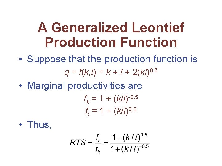
A Generalized Leontief Production Function • Suppose that the production function is q = f(k, l) = k + l + 2(kl)0. 5 • Marginal productivities are fk = 1 + (k/l)-0. 5 fl = 1 + (k/l)0. 5 • Thus,

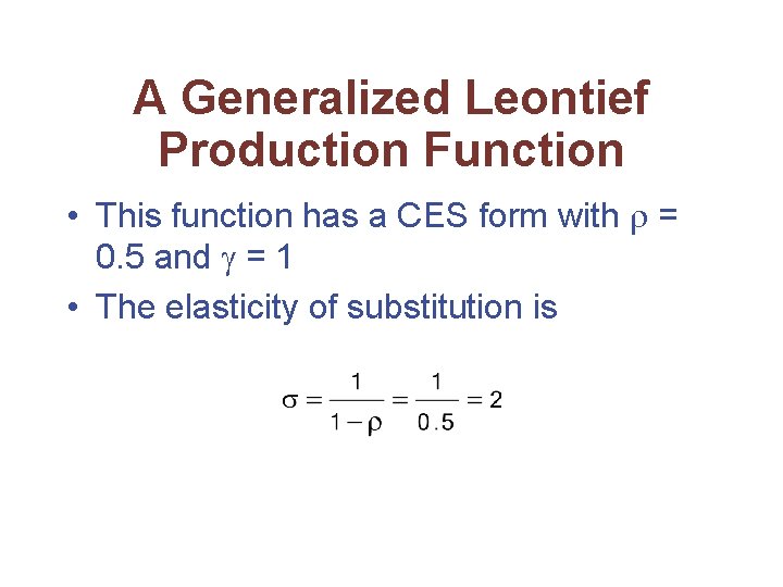
A Generalized Leontief Production Function • This function has a CES form with = 0. 5 and = 1 • The elasticity of substitution is

Technical Progress • Methods of production change over time • Following the development of superior production techniques, the same level of output can be produced with fewer inputs – the isoquant shifts in

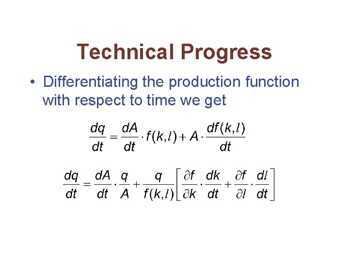
Technical Progress • Suppose that the production function is q = A(t)f(k, l) where A(t) represents all influences that go into determining q other than k and l – changes in A over time represent technical progress • A is shown as a function of time (t) • d. A/dt > 0

Technical Progress • Differentiating the production function with respect to time we get

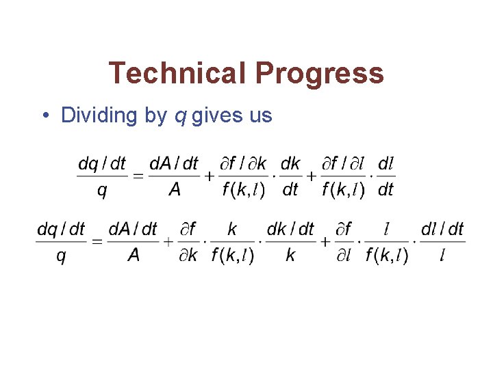
Technical Progress • Dividing by q gives us
![Technical Progress For any variable x dxdtx is the proportional growth rate in Technical Progress • For any variable x, [(dx/dt)/x] is the proportional growth rate in](https://slidetodoc.com/presentation_image/4a1d432591116b1d5d8ab2b32682fa8a/image-65.jpg)
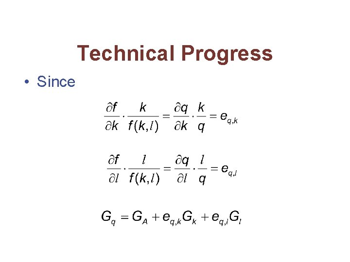
Technical Progress • For any variable x, [(dx/dt)/x] is the proportional growth rate in x – denote this by Gx • Then, we can write the equation in terms of growth rates

Technical Progress • Since

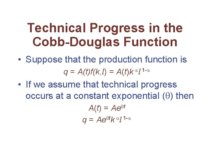
Technical Progress in the Cobb-Douglas Function • Suppose that the production function is q = A(t)f(k, l) = A(t)k l 1 - • If we assume that technical progress occurs at a constant exponential ( ) then A(t) = Ae t q = Ae tk l 1 -

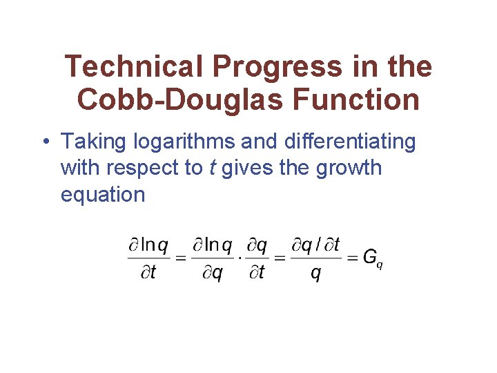
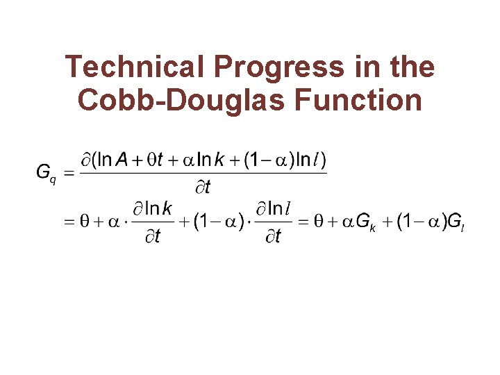
Technical Progress in the Cobb-Douglas Function • Taking logarithms and differentiating with respect to t gives the growth equation

Technical Progress in the Cobb-Douglas Function

Important Points to Note: • If all but one of the inputs are held constant, a relationship between the single variable input and output can be derived – the marginal physical productivity is the change in output resulting from a one-unit increase in the use of the input • assumed to decline as use of the input increases

Important Points to Note: • The entire production function can be illustrated by an isoquant map – the slope of an isoquant is the marginal rate of technical substitution (RTS) • it shows how one input can be substituted for another while holding output constant • it is the ratio of the marginal physical productivities of the two inputs

Important Points to Note: • Isoquants are usually assumed to be convex – they obey the assumption of a diminishing RTS • this assumption cannot be derived exclusively from the assumption of diminishing marginal productivity • one must be concerned with the effect of changes in one input on the marginal productivity of other inputs

Important Points to Note: • The returns to scale exhibited by a production function record how output responds to proportionate increases in all inputs – if output increases proportionately with input use, there are constant returns to scale

Important Points to Note: • The elasticity of substitution ( ) provides a measure of how easy it is to substitute one input for another in production – a high implies nearly straight isoquants – a low implies that isoquants are nearly L -shaped

Important Points to Note: • Technical progress shifts the entire production function and isoquant map – technical improvements may arise from the use of more productive inputs or better methods of economic organization