Predictive Models of Realized Variance Incorporating Sector and

Predictive Models of Realized Variance Incorporating Sector and Market Variance Haoming Wang April 16 th 2008

Motivation • We’ve seen that the realized variance of equities exhibits correlation with lagged daily, weekly, and monthly realized variance. • We know that equity returns are also correlated with market returns, what kind of correlation do equity variance levels have with market variance levels? • Further, it’s intuitive that the returns of individual equities are also correlated with the returns of companies in their own sector. What kind of correlation should we see with sector volatilities? • Examined regressions for pharmaceuticals and banks in the S&P 100.

Pharmaceutical Stocks • There are five companies in the S&P 100 classified as in the “Major Drugs” sector. • ABT – Abbott Labs • BMY – Bristol Myers Squibb • JNJ – Johnson & Johnson • MRK – Merck • PFE - Pfizer

Bank Stocks • Six companies in S&P 100 classified as money center banks. • BAC – Bank of America • BK – Bank of New York-Mellon • C – Citigroup • JPM – JP Morgan Chase • USB – US Bancorp • WFC – Wells Fargo

Motivation for Stock Choices • Want to choose two industries that were pretty different to see if my results weren’t just unique to the pharmaceuticals industry. • The bank industry and the pharmaceuticals industry seemed pretty different from each other. • Five pharmaceutical stocks have an average beta factor of 0. 652. • Six bank stocks have an average beta factor of 0. 945.

Background Mathematics • Realized variation (where rt, j is the log-return): • Realized sector variation: An average of daily realized variation for same sector stocks in the S&P 100 excluding whichever stock is being regressed. • Realized sector portfolio variance: average of daily stock prices is used as the price of the portfolio.

Background Mathematics • Realized variation (where rt, j is the log-return): • Realized semi-variance (where 1 is the indicator function that the return is negative) :

Background Mathematics • Further, according to BNKS, the realized semivariance converges to half the bipower variation plus negative squared jumps, or:

HAR-RV Model • The multi-period normalized realized variation is defined as the average of one-period measures, or: • The daily hetereogeneous autoregressive realized variance (HAR-RV) model of Corsi (2003) is used with daily, weekly, and monthly periods:

HAR-RV Model • The above regression is for day ahead predictions, also looked at week-ahead and month-ahead regressions. • Finally, I looked log-log regressions, where the natural log of realized variance is regressed on the natural log of the regressors. • This gives an intuitive meaning: a 1% change in the regressors implies a β% change in the dependent variable.

Extended HAR-RV model • Added sector variance for daily, weekly, and monthly periods. • For example, the RV of PFE would be regressed on the average RV of ABT, BMY, JNJ, and MRK. • What happens when PFE RV is also included in the average? • The standard errors and R-squared remain the same; however, the interpretation is not as clear. • Further, the interpretation is trickier since the stock coefficient is incorporated into the sector coefficient. • Also included the RV of the S&P 500.

Sector As A Portfolio? • Investigated constructing a portfolio of the industry. • Across the board there’s higher standard errors and lower R-squared. • I decided to stick with using an average of the sector’s realized variance.

Data Range • Data for all 11 stocks and the S&P were gathered from 1997 to 2007. • 2606 trading days worth of observations for pharmaceuticals stocks. • 2519 trading days worth of observations for the bank stocks.

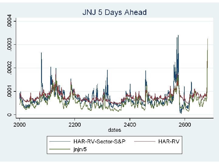
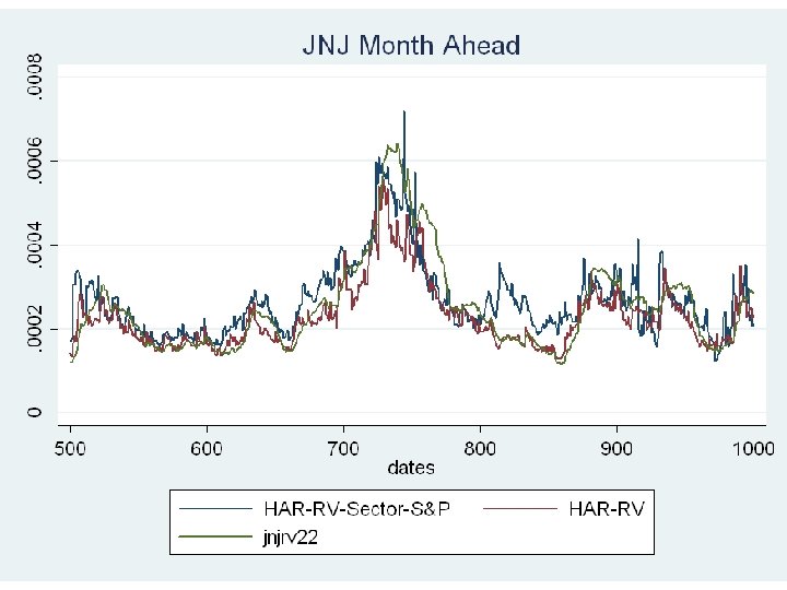
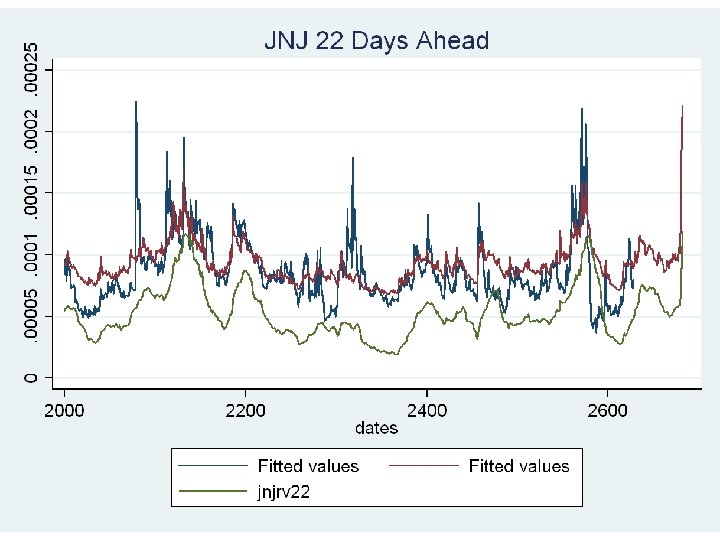
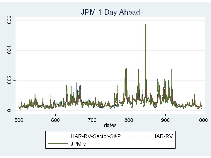
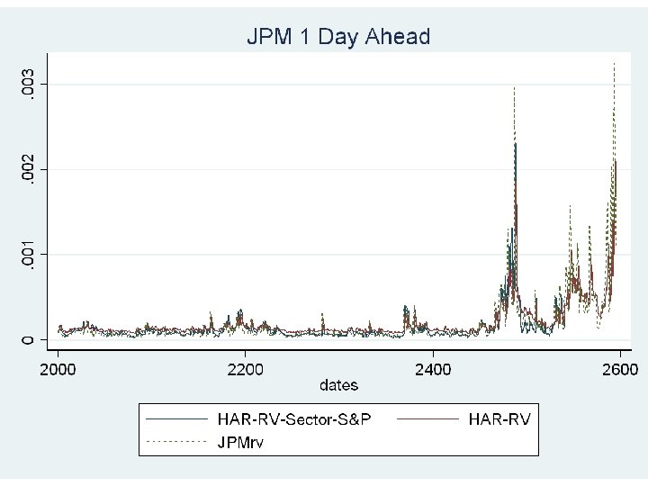
Results • We’ll focus on two companies: Johnson & Johnson (JNJ) and JP Morgan (JPM), one for each sector. • I’ve picked these two out because they show the greatest benefit from the inclusion of more regressors, but I’ll include averages as well.

R-Squared JNJ Day Ahead Week Ahead Month Ahead HAR-RV 47. 22% 54. 57% 49. 44% HAR-RV-Sector 55. 39% 63. 52% 54. 89% HAR-RV-S&P 53. 48% 61. 61% 52. 01% HAR-RV-Sector. S&P 56. 74% 65. 65% 57. 42% % Increase (HARRV to HAR-RVSector-S&P) 9. 52% 11. 08% 7. 98%

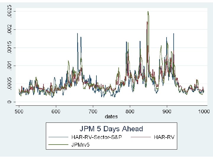
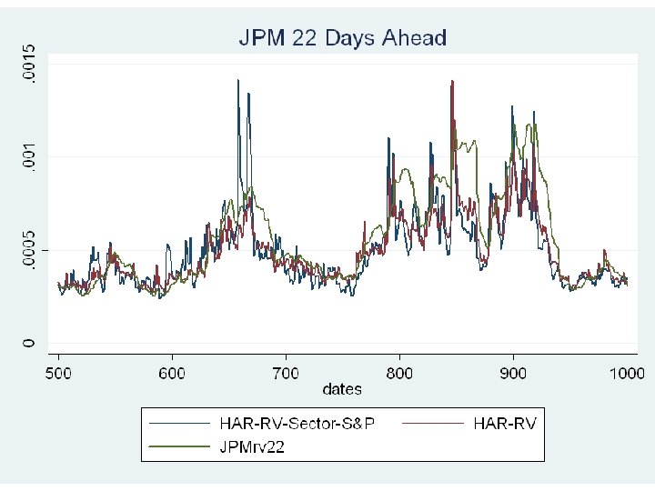
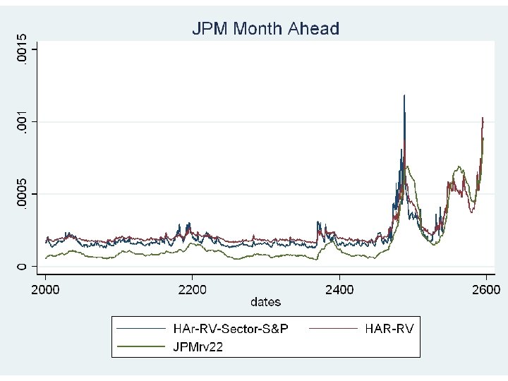
R-Squared JPM Day Ahead Week Ahead Month Ahead HAR-RV 47. 73% 44. 33% 43. 15% HAR-RV-Sector 54. 30% 58. 37% 49. 77% HAR-RV-S&P 54. 24% 56. 73% 50. 60% HAR-RV-Sector. S&P 55. 98% 61. 58% 51. 92% % Increase (HAR -RV to HAR-RVSector-S&P) 8. 25% 17. 25% 8. 77%

Analysis • We see marked increases in the explanatory power of the regression model, with the greatest improvement in the weekly predictions. • This makes intuitive sense: it should be easier to predict smoothed out variance measures. • This is in line with the level of the R-squared: we have the highest level of R-squared in the weekly predictive model. • Seems intuitive that the model with the highest explanatory power should also see the most improvement.

Analysis • In the pharmaceuticals sector, we see an average increase in R-squared of 5. 12% for daily predictions, 5. 80% for weekly predictions, and 6. 41% for monthly predictions. • In the banking sector, we see an average increase in R-squared of 6. 24% in daily predictions, of 6. 83% for weekly predictions, and 3. 41% for monthly predictions.

Coefficient Estimates and Significance βCD βCW βCM Day Ahead 0. 1684*** -0. 0297 0. 4480** JNJ Week Ahead 0. 08991* -0. 0033 0. 4942* Month Ahead 0. 0373 -0. 0035 0. 5028* βSD βSW βSM 0. 2385*** 0. 1462 -0. 1351 0. 1503*** 0. 2376* -0. 0673 0. 0947*** 0. 1987 0. 1451 βSPD βSPW βSPM 0. 1202 0. 4976 -0. 5412* 0. 2664* 0. 0413 -0. 5033* 0. 1101* -0. 0668 -0. 6934** β 0 -0. 000003 0. 000006 0. 000027 * P<0. 05, **p<0. 01, ***p<0. 001

Coefficient Estimates and Significance βCD βCW βCM Day Ahead 0. 3680*** -0. 0901 0. 3273*** JPM Week Ahead 0. 0998*** -0. 0282 0. 3833* Month Ahead 0. 0219 0. 0261 0. 4340** βSD βSW βSM 0. 3399* 0. 2906 -0. 6664* 0. 6399** -0. 1623 -0. 5302* 0. 2939*** -0. 2043 -0. 0369 βSPD βSPW βSPM 0. 3479 0. 6073 0. 5866 0. 1251 1. 129 0. 6116 0. 1195 1. 209 -0. 6032 β 0 -0. 000004 0. 0000226 0. 000099*** * P<0. 05, **p<0. 01, ***p<0. 001

F-Test JNJ JPM Day Week Month Sector 0. 0000 0. 0001 0. 0008 0. 0001 S&P 0. 0984 0. 0531 0. 0062 0. 0929 0. 5355 0. 456 P-Value

Analysis • In all regressions we see that the lagged daily sector variance is strongly significant. • There are clear sector effects at work, although only the previous day sector RV seems to play a consistently statistically significant role. • However, sector regressors are jointly significant for all time horizons. • While the p-values for the sector regressors remains at around the same level, it’s interesting to note that for JNJ the S&P regressors become much more significant as the horizon increases, perhaps suggesting that market effects play out in a longer time-frame for JNJ.

Analysis • The S&P coefficients are harder to interpret: there are no clear patterns in significance, although daily and monthly S&P regressors seem to be significant for JNJ, however, there is still the weirdness of negative coefficients. • JPM is especially strange because the sign of the monthly S&P lag flips signs. • From looking at semi-variances, this seems to be driven by high upward semi-variance. • However, we do have a pretty clear pattern: the previous day’s sector RV does seem to be an important driver of realized variance.

Analysis • Increasing the time horizon also doesn’t seem to solve the problem of the negative monthly coefficients. • I’ll talk about this later, but what effect does the time-frame have on the model’s coefficients? • I plan on investigate this further for next semester.

Analysis • It’s also interesting to note that even with the inclusion of the S&P and sector, we still see the same-stock daily lags decreasing in importance as the time horizon increases and the monthly lags increasing in importance. • Further, the weekly lag seems to be relatively unimportant. It seems that the most important drivers are the short term and the long term. • For JNJ we see some intuitive results for the sector and the stock: the lagged daily effects grow weaker as the prediction horizon increases and the monthly effects are stronger.

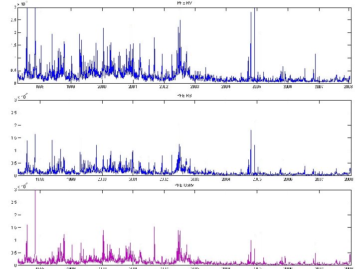
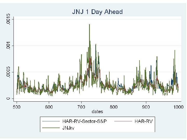
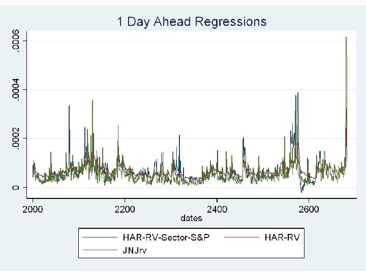
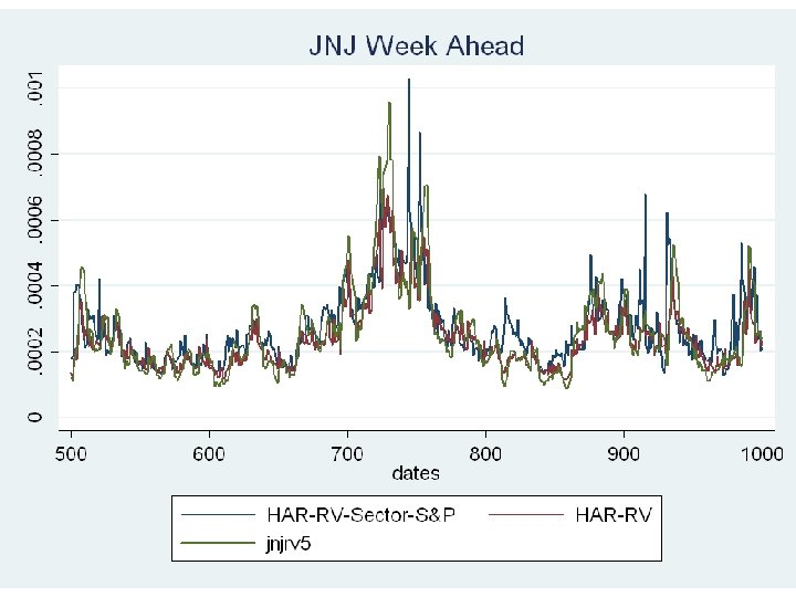
Analysis • It’s interesting to note the patterns in RV predictions. • Regression models with sector and S&P realized variance seem to have much greater ability to exhibit spikes in realized variance. • This makes intuitive sense: it’s likely that events which cause spikes in volatility for the market or the sector to be associated with spikes in a specific stock.

Analysis • It’s also interesting to note trends in realized variance over this data set. The first graph is from about 1999 -2001 and the second graph is from 2006 -2008. • Day ahead predictions seem close for both time periods. • However, for the early part of 2006 -2008 (pre-credit crisis) the model consistently over-predicts week ahead and month ahead realized variance. • It seems that 2006 -2007 was a period of below average volatility in the market. • It would be interesting to see how the model changes for different periods of data corresponding to different volatility regimes.

Extensions For Next Semester • Breaking up realized variance into continuous and jump components for both the sector and stock:

Extensions For Next Semester • Including the sector and S&P realized variances seems to increase the prediction of spikes in realized variance, it would be interesting to see how the inclusion of jumps as regressors changes these dynamics. • Further investigation using semi-variance of the negative coefficient in monthly lags.