Predictive Regression Models of Realized Variation and Realized

Predictive Regression Models of Realized Variation and Realized Semi-Variance in the Pharmaceuticals Sector Haoming Wang 2/27/2008

Introduction • Want to examine predictive regressions for realized variance and realized semi-variance (variance caused by negative returns). • Sector realized variance and realized semivariance is introduced as a regressor. • Regressions are of the form of the HAR-RV regression talked about in Anderson, Bollerslev, and Diebold (2005). • Semi-variance taken from Barndorff-Nielsen, Kinnebrock, Shephard (2008)

Introduction • Will first address HAR-RV regressions featuring sector RV. • Then, will examine Barndorff-Nielsen, Kinnebrock, Shephard (BNKS) work on realized semi-variance and possible HAR-RS regressions.

Background Mathematics • Realized variation (where rt, j is the log-return): • Realized sector variation: An average of daily realized variation for ABT, BMY, JNJ, MRK, and PFE, excluding whichever stock is being regressed.

HAR-RV Model • The multi-period normalized realized variation is defined as the average of one-period measures, or: • The daily hetereogeneous autoregressive realized variance (HAR-RV) model of Corsi (2003) is used with daily, weekly, and monthly periods:

Extended HAR-RV model • Added sector variance for daily, weekly, and monthly periods. • For example, the RV of PFE would be regressed on the average RV of ABT, BMY, JNJ, and MRK. • Examined regressions for ABT and PFE.

OLS vs. Robust Regression • The pricing data most likely has leverage points (data points that have an extremely large effect on the coefficient estimates) as well as sampling errors (trading days that were removed). • This could create small disturbances for the data which are hard to isolate. • Thus, standard OLS regression might not be the best way to estimate these coefficients since OLS is sensitive to leverage points.

Leverage Point Example

OLS vs. Robust Regression • Thanks to Fradkin (2007) we can mitigate these problems by using robust regressions instead of OLS regressions. • The “rreg” command in STATA is used, which iteratively reweighs least squared based on Mestimators. • Robust regressions will be compared with OLS regressions in the following slides.

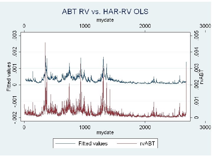
ABT Regression Results • R-squared of 0. 5126 in line with averages seen in Fradkin (2007). • All three coefficients are statistically significant and contribute about the same to the RV prediction. • A unit increase in daily realized volatility will imply on average an increase of. 3312 +. 2935/5 +. 2887/22 = 0. 4030

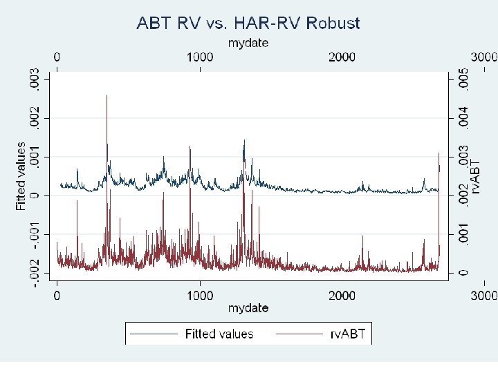
ABT Regression Results • Standard errors decrease across the board, although the coefficients for daily and weekly RV decrease. • A increase in daily RV implies on average an increase in predicted RV of 0. 3167, about 75% of the predicted OLS regression.

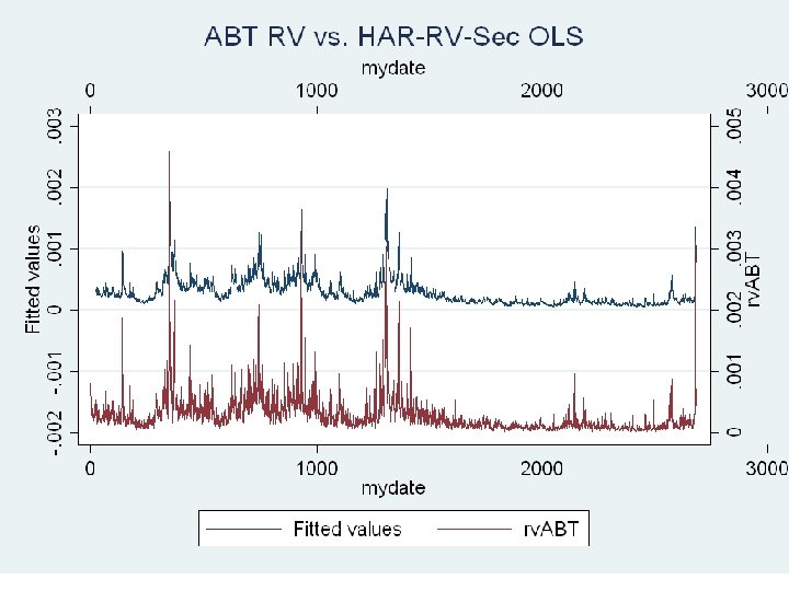
ABT Regression Results • Coefficients of lagged RV remain statistically significant and largely have the same values. U nit increase in daily RV on average produces an increase in RV of 0. 3734. • The only coefficient that appears to be significant is the previous day average sector RV. U nit increase in daily average sector RV seems to have a very small effect on RV. • R-squared does increase by a very small amount.

ABT Regression Results • These results mirror the jump to robust regression from the HAR-RV regression. • Coefficients and standard errors all decrease. • U nit increase in daily realized variation only expected on average to increase the RV prediction by 0. 2614.

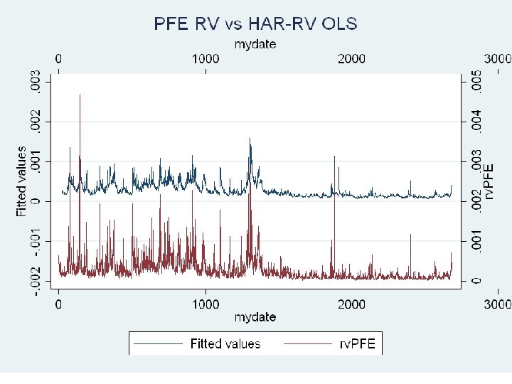
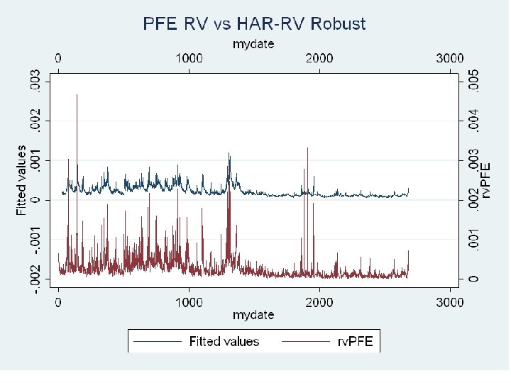
PFE Regression Results • Again we have highly significant coefficients, although the R-squared is lower than ABT. • A unit increase of RV on average implies an increase in next day RV of 0. 3557.

PFE Regression Results • Once again we see much lower standard errors along with a decrease in the coefficients. • Previous 5 -day RV seems to be affected the most • A unit increase in RV on average implies an increase in the next day’s RV of 0. 2702

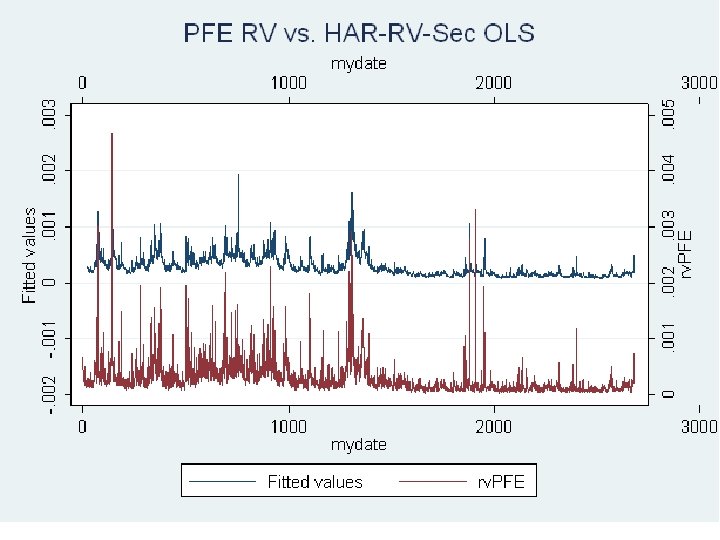
PFE Regression Results • Some interesting things happen when we add sector RV to this regression. We see that standard errors increase across the board. • Coefficients of daily and weekly RV decrease, although the coefficient for monthly RV increases. • The only significant RV we see is the daily sector RV, similar to ABT. • U nit increase in daily RV implies on average an increase in predicted RV of 0. 3144

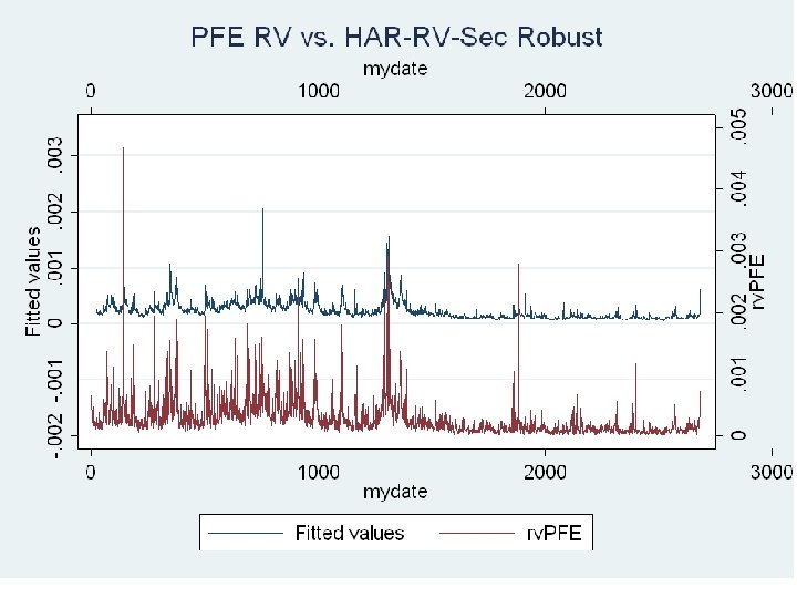
PFE Regression Results • This was the most interesting regression. Coefficients on almost all of the regressors change significantly from before. Once again, standard errors are lower across the board. • Daily sector RV actually becomes the most important coefficient. Further, all coefficients are now statistically significant. • Unit increase in daily RV implies an average increase in predicted RV of 0. 2084 • Unit increase in daily sector RV implies on average an increase in predicted RV of 0. 3207, almost entirely driven by the previous day’s sector RV.

Analysis • In both ABT and PFE we see peaks and valleys in variance. 1997 -2003 corresponds to a period of high volatility. • 2003 -2008 seems to have relatively low volatility. • Perhaps it would be better to split the data and perform separate regressions?

Analysis • Extreme spikes in RV are unsurprisingly extremely hard to predict, although periods of high RV are easily seen. • The low R-squared for PFE could be explained by the large number of volatility spikes from 1997 -2003 in the data. • As a whole, monthly realized variation seems to have a large effect relative to the coefficient for the S&P 500 from Bollerslev 2005

Analysis • Switching to robust regressions consistently lower standard errors though other effects are never too pronounced. • The outlier is in the case of PFE, where the robust regression of HAR-RV-Sector is drastically different from the OLS regression.

Analysis • Introducing sector-RV doesn’t seem to have any meaningful improvement on fit, although for both ABT and PFE the previous day’s sector average RV is significant. • The most interesting case is the robust regression for PFE with lagged RV and lagged sector RV. • For ABT, including sector RV seems to help with predicting some spikes in RV.

Realized Semi-Variance

Background Mathematics • Realized variation (where rt, j is the log-return): • Realized semi-variance (where 1 is the indicator function that the return is negative) :

Background Mathematics • Further, according to BNKS, the realized semivariance converges to half the bipower variation plus negative squared jumps, or:

Background Mathematics • Bipower Downward Variance: • Could we us RS and BPDV to test for downward jumps? • According to BNKS: “this is going to be hard to carry out solely based on in-fill asymptotics without stronger assumptions than we usually like to make due to the presence of the drift term in the limiting result and the non-Mixed Gaussian limit theory”.

Background Mathematics • According to BNKS we could perform jump testing if we assumed the drift term to be 0 and that there was no leverage term. • What does this mean?

Background Mathematics • Suppose we separate the squared returns into a matrix of their up and down components: • Then suppose that the log prices form a semi-martingale Brownian process (first term is drift) and an included jump component : so that:

Background Mathematics • For the above the left hand side should just be the bipower variation (continuous component of variance) plus the squared positive jumps and negative jumps. • At this point I was unable to understand the rest of the proof. BNKS make use statistical theory beyond my grasp along with Kinnebrock and Pdolskij (2007) to show that V(Y, n) converges in distribution to a mixed Gaussian distribution:

Background Mathematics • The presence of the drift term in the limiting distribution is why jump testing for downside jumps is tricky. • If the drift term is equal to zero, then we can construct confidence intervals/conduct hypothesis testing. However, when the drift term is non-zero, the limiting result is biased. • Thus we would have to assume that the drift term was zero to conduct jump testing.

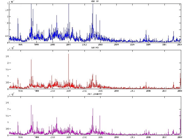
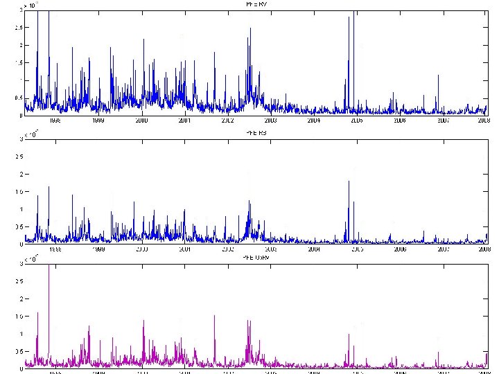
Realized Variation Decomposition (PFE)

Persistence of RS Coefficients ABT OLS ABT Robust PFE OLS PFE Robust RV-1 0. 3089 0. 1705 0. 2693 0. 1896 RS-5 0. 2304 0. 2244 0. 1405 0. 09 RV-22 0. 3433 0. 2889 0. 4426 0. 3189 • Lagged 22 day realized semi-variance has the greatest impact on implied future volatility. • Qualitative reasoning for the high value placed on monthly realized semi-variance?

HAR-RV Extensions • Include jumps into regressions, use HAR-RV-CJ regression. • How should I include sector jumps? Indicator if any company in the sector has a jump? • Examine the RAV regression used in Fradkin 2007.

Realized Semi-variance Extensions • In the vein of RAV, how about semi-RAV? Not sure if econometrically feasible, but seems that I could add an indicator just like in semi-RV calculations. • Persistence of downside variation? According to traders: volatility is higher on average in a down market than in an upward moving market. • Connect to implied volatility? In a downward market volatility/options is expensive • Regress RV on RS.