Population Ecology Population Demography Ways of Expressing Population

Population Ecology Population = Demography =

Ways of Expressing Population Growth • Net birth rate = Births per unit time • Net death rate = Death per unit time • Net population increase = Net Birth rate – Net Death rate • World Population mid-year 2007 • 6. 625 billion people – – Net birth rate/ year = 139, 125, 000 Net death rate/year = 59, 625, 000 Net Increase/year = 78, 500, 000 USA Population mid-year 2007 = 302, 200, 000 • World Increase = USA Population - 3. 85 years

Expressing Population Growth • Births/1, 000 = • (Births per year/ mid-year population size) X 1, 000 • Deaths/1, 000 = • (Death per year /mid-year population size) X 1, 000 • Natural Rate of Increase = • Births/, 1000 – Death/1, 000

World Population mid-year 2007 • • Birth rate = 21 Death rate = 9 Rate of Natural Increase = 12 Percent Growth = – 1. Rate of Natural Increase/10 – 2. 12/10 = 1. 2% • Approximate doubling time = • 70 years/ % Growth • World Doubling Time =70 yrs/1. 2 % = 58 yrs

Comparison of Ways to Express Population Growth A. Population size = 1, 000 B. Population size = 1, 000 1. Net birth = 10 Net births = 100 2. Net deaths = 50 3. Net increase = 50 1. Birth /1000 = 10 = 0. 10 2. Death/1000 = 5 = 0. 05 3. Rate of natural increase = 5 = 0. 05 4. % growth = 0. 5% = 0. 005%

Rate of Natural Increase and % Growth do not include net immigration • • • United States Birth per 1000 = 14 Deaths per 1000 =8 Net Immigration per 1000 =4 % Growth with Immigration = 18 -8 = 1. 0% % Growth w/o immigration = 14 -8 = 0. 6%

Population Growth (Basic Growth Curves) • “J-shaped” growth or exponential growth • Sigmoid or “S-shaped” growth

J-shaped or exponential growth curve EXPONENTIAL GROWTH Population Size LAG BEND TIME

EXPONENTIAL GROWTH • Population increase – Fixed percentage of population size at the beginning of the period • Example of exponential growth is geometric growth – Growth by doubling – Fixed percentage is 200 percent

Geometric Growth of a Sheet of Paper • • • Number of doubles 1 2 3 4 5 6 7 8 Thickness 2/254 inch 4/254 8/254 16/254 32/254 64/254 128/254 256/254

Geometric Growth of a Sheet of Paper • • • Number of doubles 12 20 35 42 • 50 Thickness 1. 25 foot 340 feet 3, 000 miles 384, 000 miles (reaches the moon) 93, 000 miles (reaches the sun)

Exponential Growth • Initially, no limit placed on growth • Population grows at max possible rate – Intrinsic growth rate (biotic potential) • r = biotic potential • Maximum rate/individual • Growth is halted abruptly: – Depleted resource (food or space) – Epidemic disease • Environmental resistance – Applied all at once

J-shaped Growth Curve POPULATION SIZE Carrying Capacity Environmental resistance – applied abruptly Time

J-shaped growth curves are characteristic of populations in environments of • Low diversity • Few predators or competitors (few ecological controls) • Simple food webs

Sigmoid or S-shaped Growth Curve Biotic Potential Carrying Capacity Population Size Time

Sigmoid Curve • Detrimental factors (environmental resistance) – Increases in proportion to population increase • Characteristic of environment – High diversity – Predators, competitors exert biological control

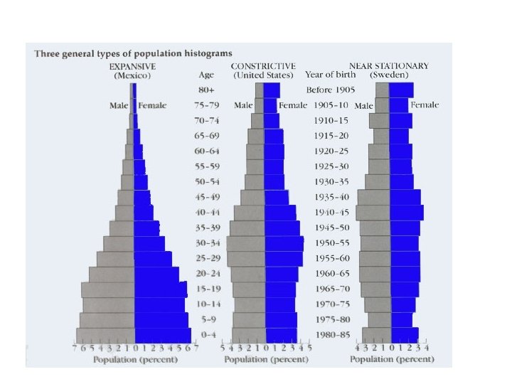
AGE STRUCTURE DIAGRAMS • Graphically – % of individuals within various age categories • Three age categories • Prereproductive (Age 0 -14 years) • Reproductive (Age 15 -44 years) • Postreproductive ( Age 45+) • Plot males on left and females on right

Age Structure Diagrams Reproductive Pre-reproductive Younger to older Post-reproductive Age % males in the % females in the age group

What Does the Age Structure Diagram Indicate? • Growth Patterns • Proportional Distribution in Age Categories

Three general types of age structure diagrams • Expanding • Stabilizing • Diminishing

Expanding Growth 2. 7% Postreproductive Reproductive Prereproductive Stabilizing 0. 6% Diminishing – 0. 2%

Changes in USA Age Structure • Last century USA – Expanding population to a stabilizing population – Total fertility rate (2007 USA 2. 1) • Post war baby boom (1946 and 1964) – Peaked 1955 -1959 – 75 million bulge in population – Large affect on social and economic structure

Effect of Post War Baby Boom • 1960 -1975 – expansion of schools • Late 1970’s – 1980’s high unemployment • 2, 005 -2025 – Dominance of middle age (Pension cost begin to rise) • 2, 025 – 2, 040 – Period of Senior Citizens

Changes -USA Birth Rates and Death Rates • • • Year BR DR RNI %Growth 1947 26. 6 15. 0 11. 6 1. 16 1977 14. 7 9. 0 5. 7 0. 57 1987 16. 0 9. 0 7. 0 0. 70 1996 14. 6 8. 8 5. 8 0. 58 2000 15. 0 9. 0 6. 0 0. 60 2004 14. 0 8. 0 6. 0 0. 60 2007 14. 0 8. 0 6. 0 0. 60 Over the last 50 years births and death rates have declined BR = Birth Rate, DR = Rate, RNI = Rate of Natural Increase

Implications of Death Rates and Birth Declining • Fewer Births = fewer young people • Fewer Deaths = More Older People • Birth rates declined more rapidly than death rates = fewer young people more older people

Results of declining growth in USA • USA has an aging population: – Proportionately fewer young people and more older people • • • Median Age of the USA Population 1970 -- 29 years 1990 -- 33 2, 000 -- 36 2010 -- 39

United States’ Aging Population • Population 1950 • Ages 65 -84 (Millions) 11. 7 • 85 and over (Millions) 0. 6 1985 25. 8 2. 7 2020 44. 3 7. 1 • 65 and older % total 7. 7% 12% 17. 3% • Total Pop. (years) 68. 2 74. 7 78. 1 • Federal Spending • Pension & Health-care As a % of GNP 1. 6% 9. 3% 11. 8% • LIFE EXPECTANCY

Social Security • Continued adjustments in Social Security – Not a pay as you go system. – Pay while you work get benefits later • As the populations ages: – Future retirees will have few workers supporting their retirement than current retirees or retirees in the past

Ratio: retirees/worker • • • Date 1950 1965 1985 2025 Retiree/workers 1/16 1/5 1/4 1/3 1/2

Social Security: Current Status • 2018 – More expenditures than income • 2042 –Trust Fund Depleted – Pay out all in coming funds – 75 % of current benefits • Reality Trust fund is not fully funded

Suggested Solutions • Raise FICA Tax (Federal Insurance Contributions Act) – Current (7. 65%) • Tax income over $90, 000 (current cap) • Tax one-half of Social Security Income over $32, 000 • What changes have occurred?

Birth Year & Age for Full SS Retirement Benefits Birth Year Age for full benefits 1937 or earlier 65 1939 65 and 4 months 1941 65 and 8 months 1943 -1954 66 1955 66 and 2 months 1957 66 and 6 months 1959 66 and 10 months 1960 and later 67

Cunningham, Cunningham and Saigo, “Environmental Science, 8 th ed. ” Mc. Graw Hill, Fig. 7. 9

Age Distribution of the World’s Population Structures by Age and Sex, 2005 Millions Less Developed Regions More Developed Regions Age Male Female 80+ 75 -79 70 -74 65 -69 60 -64 55 -59 50 -54 45 -49 40 -44 35 -39 30 -34 25 -29 20 -24 17 -19 10 -16 5 -9 0 -4 Male Female Source: United Nations, World Population Prospects: The 2002 Revision (medium scenario), 2003. Provided online by the Population Reference Bureau Graphics Bank, The Graphics Bank was prepared by Allison Tarmann, senior editor, and Theresa Kilcourse, senior graphics designer. Please visit www. prb. org.

Examples of Age Structure Diagrams • Rapid Growth: Kenya, Nigeria, Saudi Arabia (doubling times 20 -35 years) • Slow Growth: United States, Australia, Canada (doubling times 88 -175) • Zero Growth: Denmark, Austria, Italy • Negative Growth: Germany, Bulgaria, Hungary