PATTERN RECOGNITION AND MACHINE LEARNING CHAPTER 8 GRAPHICAL

PATTERN RECOGNITION AND MACHINE LEARNING CHAPTER 8: GRAPHICAL MODELS

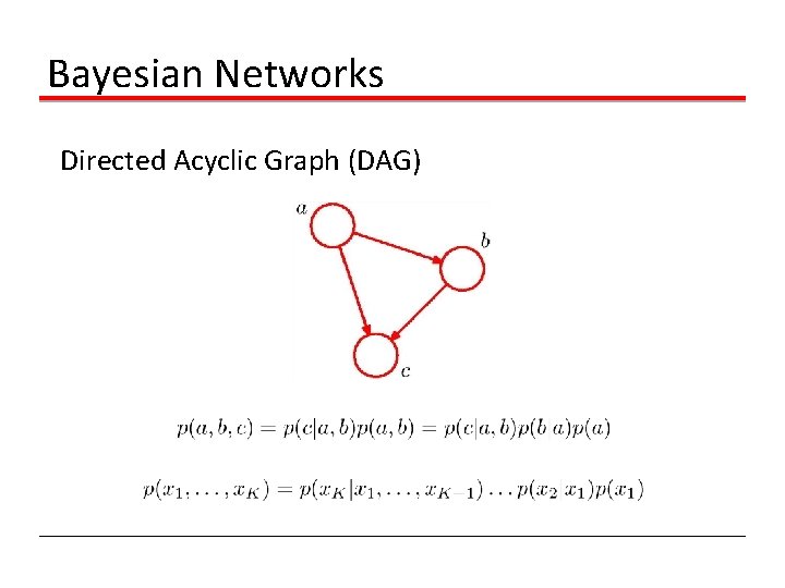
Bayesian Networks Directed Acyclic Graph (DAG)

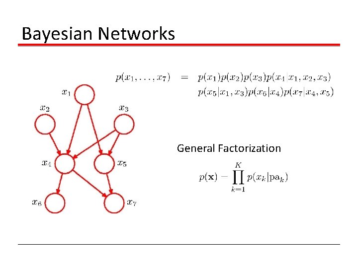
Bayesian Networks General Factorization

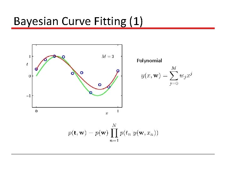
Bayesian Curve Fitting (1) Polynomial

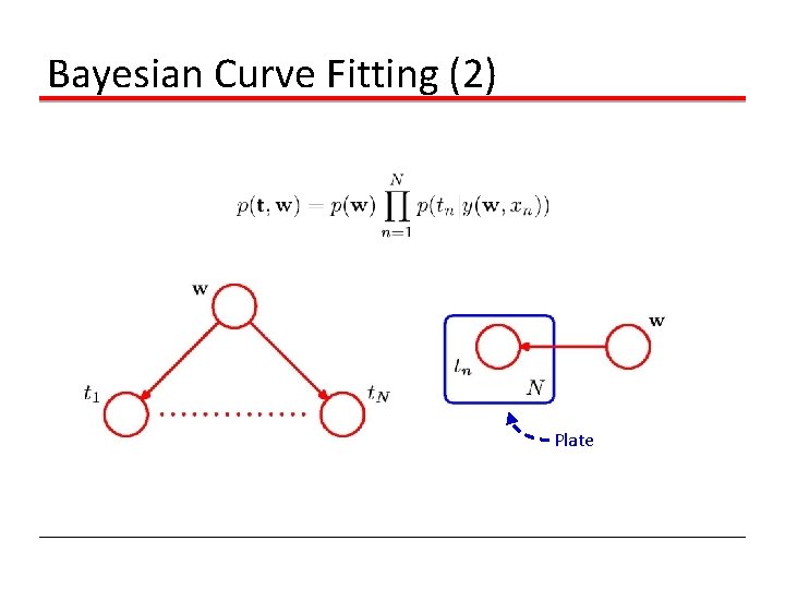
Bayesian Curve Fitting (2) Plate

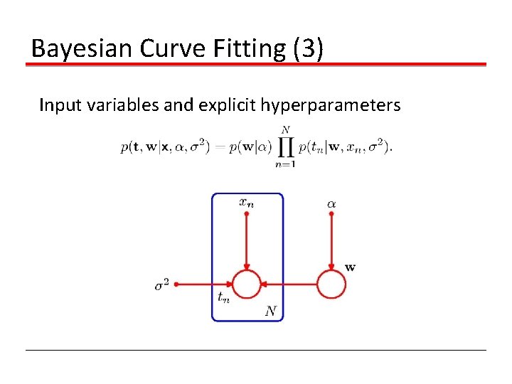
Bayesian Curve Fitting (3) Input variables and explicit hyperparameters

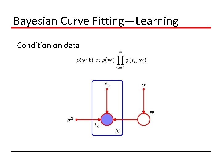
Bayesian Curve Fitting—Learning Condition on data

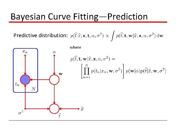
Bayesian Curve Fitting—Prediction Predictive distribution: where

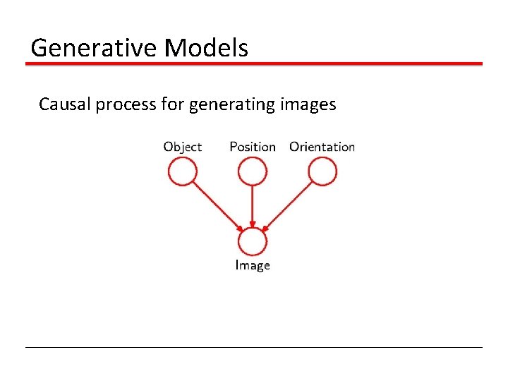
Generative Models Causal process for generating images

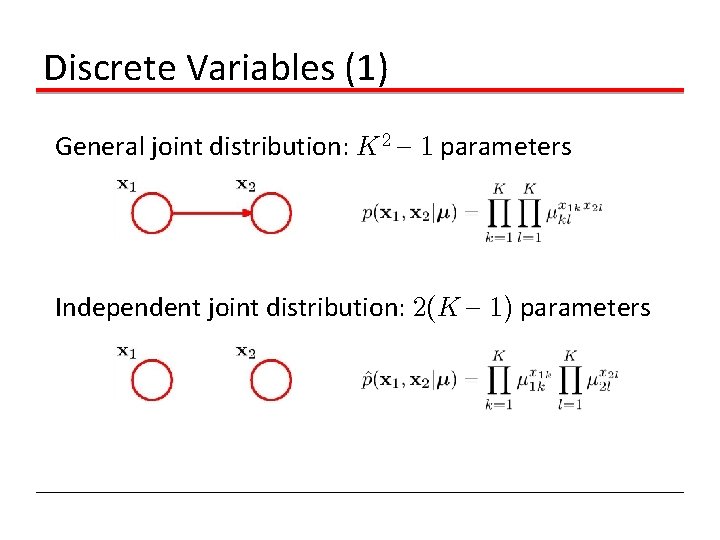
Discrete Variables (1) General joint distribution: K 2 { 1 parameters Independent joint distribution: 2(K { 1) parameters

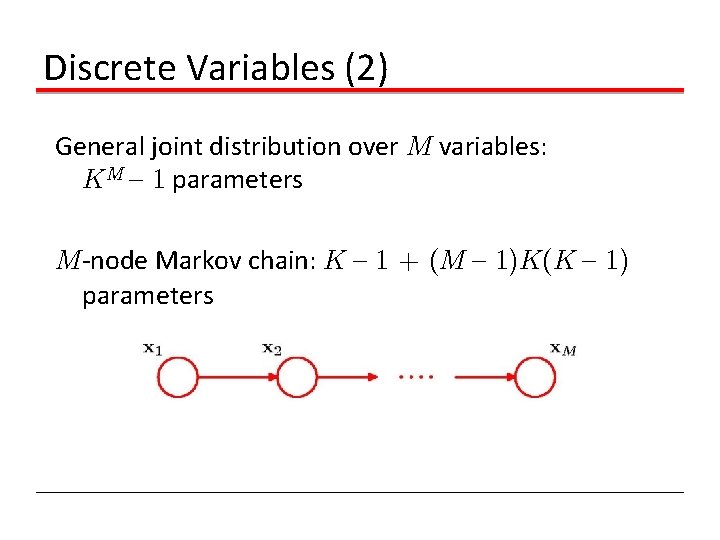
Discrete Variables (2) General joint distribution over M variables: KM { 1 parameters M-node Markov chain: K { 1 + (M { 1)K(K { 1) parameters

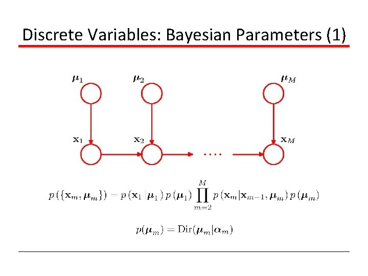
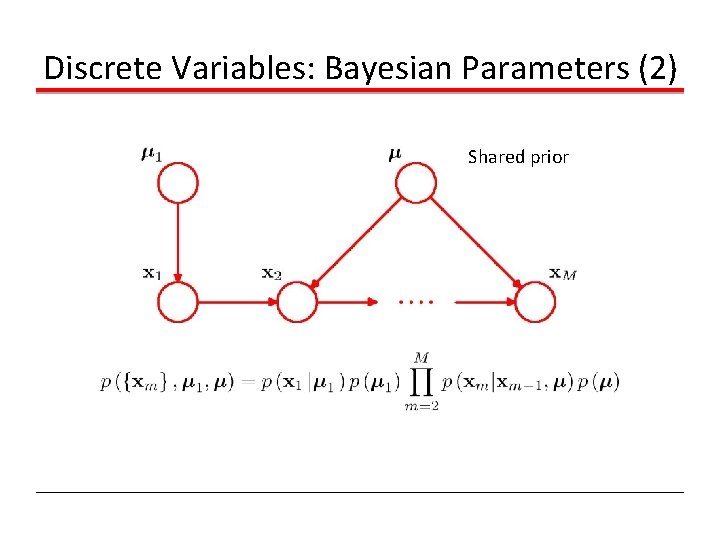
Discrete Variables: Bayesian Parameters (1)

Discrete Variables: Bayesian Parameters (2) Shared prior

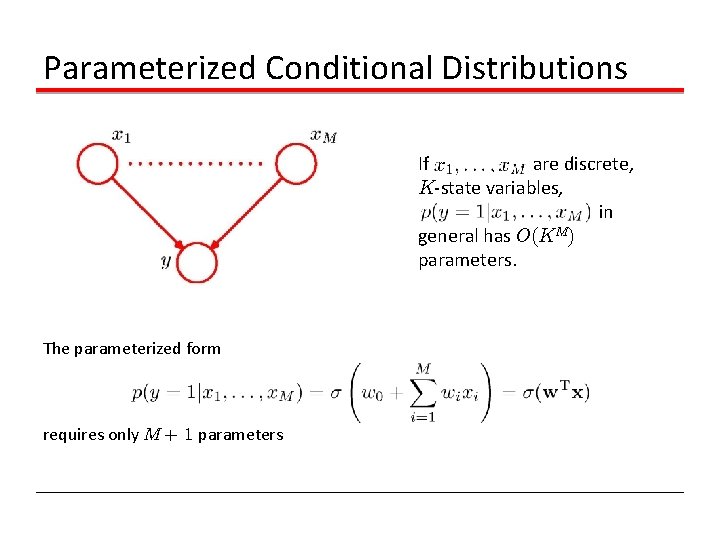
Parameterized Conditional Distributions If are discrete, K-state variables, in general has O(KM) parameters. The parameterized form requires only M + 1 parameters

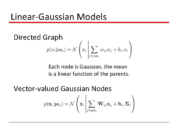
Linear-Gaussian Models Directed Graph Each node is Gaussian, the mean is a linear function of the parents. Vector-valued Gaussian Nodes

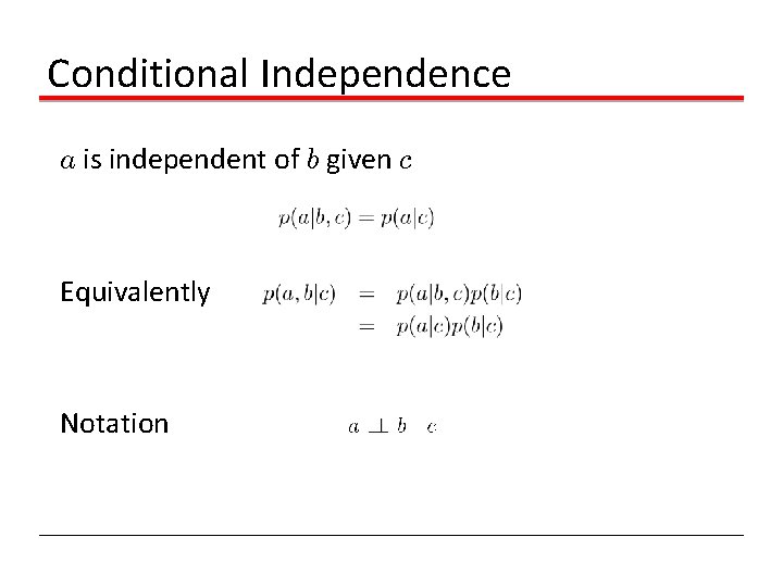
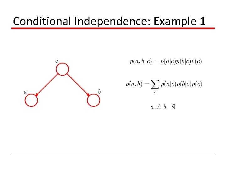
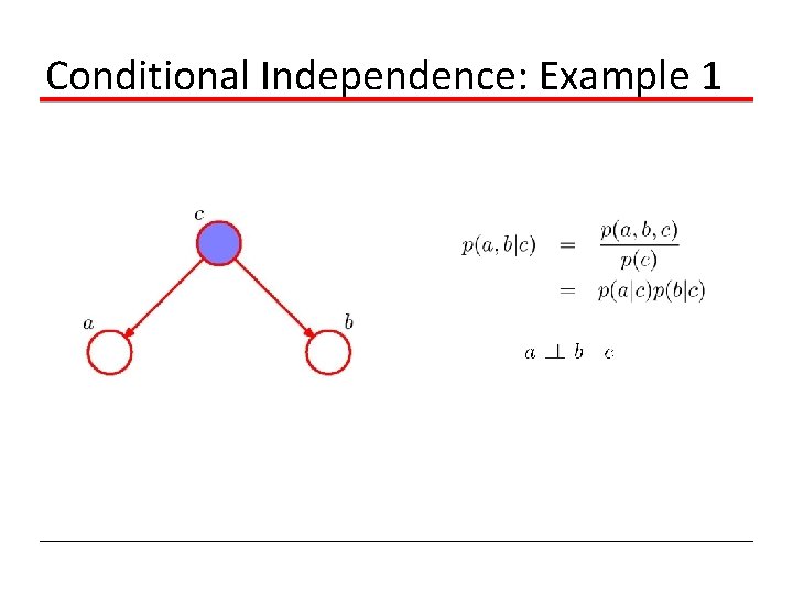
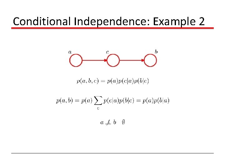
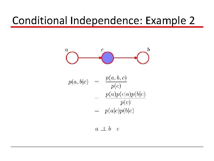
Conditional Independence a is independent of b given c Equivalently Notation

Conditional Independence: Example 1

Conditional Independence: Example 1

Conditional Independence: Example 2

Conditional Independence: Example 2

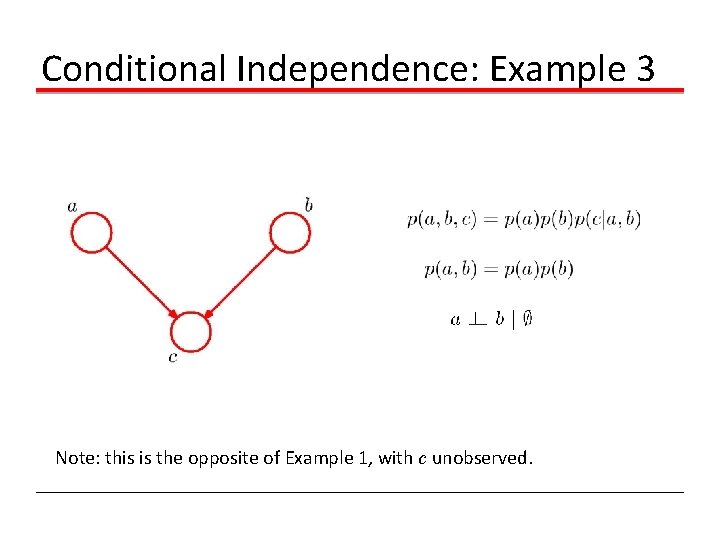
Conditional Independence: Example 3 Note: this is the opposite of Example 1, with c unobserved.

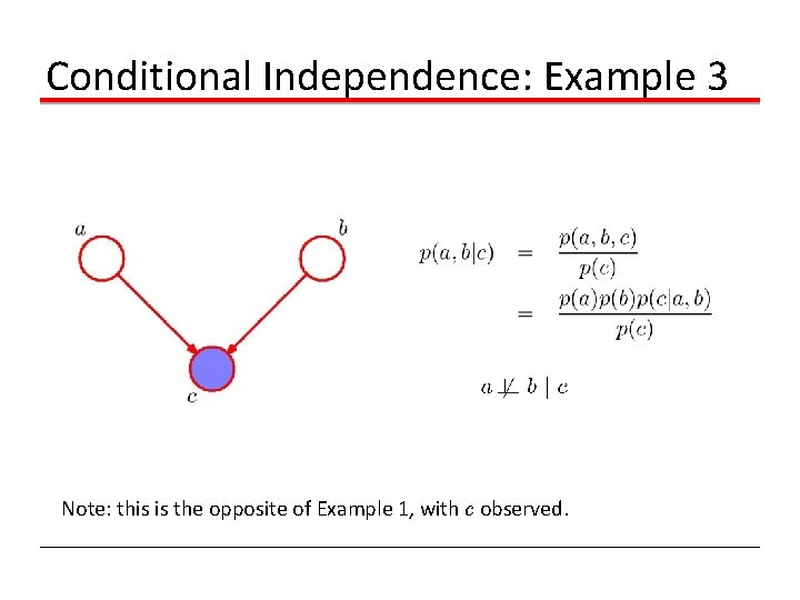
Conditional Independence: Example 3 Note: this is the opposite of Example 1, with c observed.

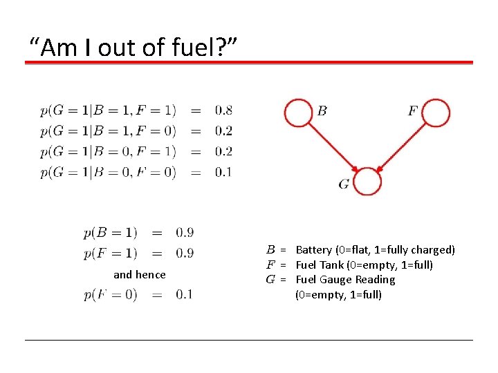
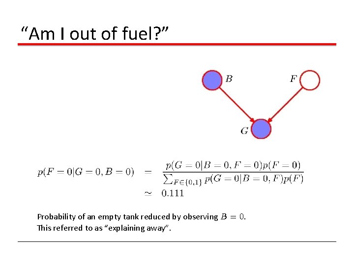
“Am I out of fuel? ” and hence B = Battery (0=flat, 1=fully charged) F = Fuel Tank (0=empty, 1=full) G = Fuel Gauge Reading (0=empty, 1=full)

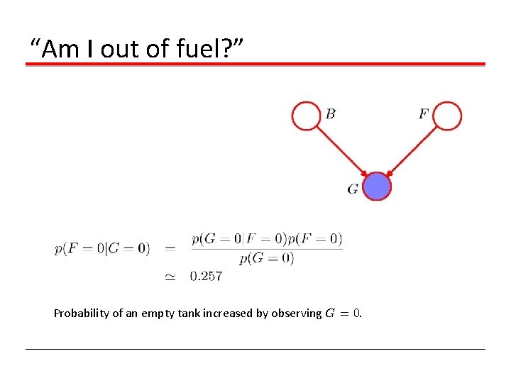
“Am I out of fuel? ” Probability of an empty tank increased by observing G = 0.

“Am I out of fuel? ” Probability of an empty tank reduced by observing B = 0. This referred to as “explaining away”.

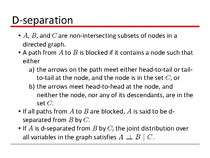
D-separation • A, B, and C are non-intersecting subsets of nodes in a directed graph. • A path from A to B is blocked if it contains a node such that either a) the arrows on the path meet either head-to-tail or tailto-tail at the node, and the node is in the set C, or b) the arrows meet head-to-head at the node, and neither the node, nor any of its descendants, are in the set C. • If all paths from A to B are blocked, A is said to be dseparated from B by C. • If A is d-separated from B by C, the joint distribution over all variables in the graph satisfies.

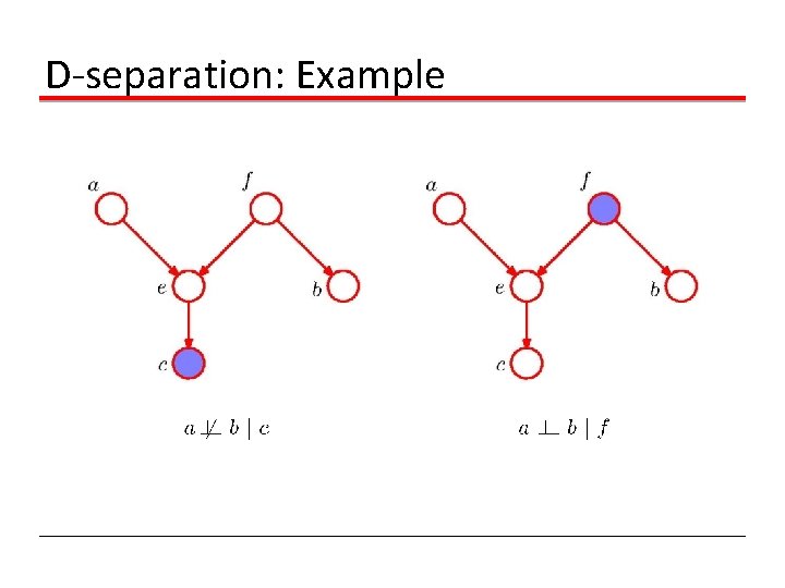
D-separation: Example

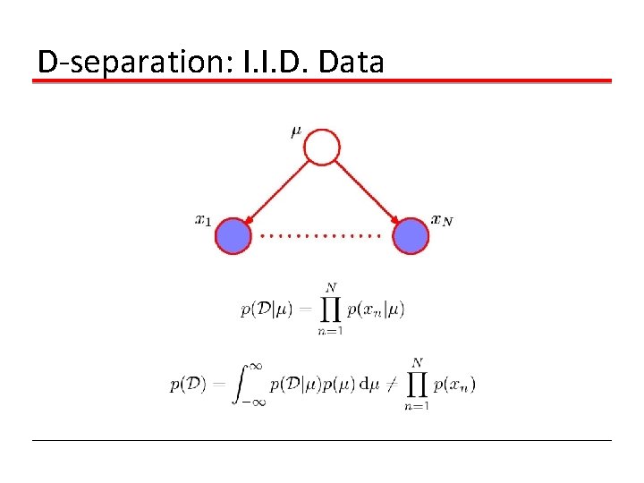
D-separation: I. I. D. Data

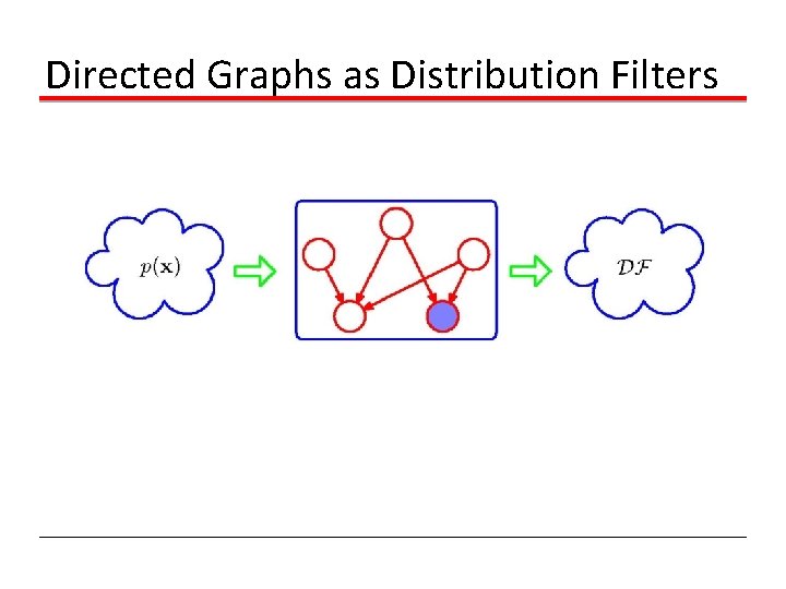
Directed Graphs as Distribution Filters

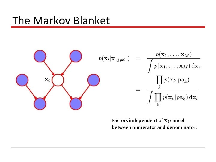
The Markov Blanket Factors independent of xi cancel between numerator and denominator.

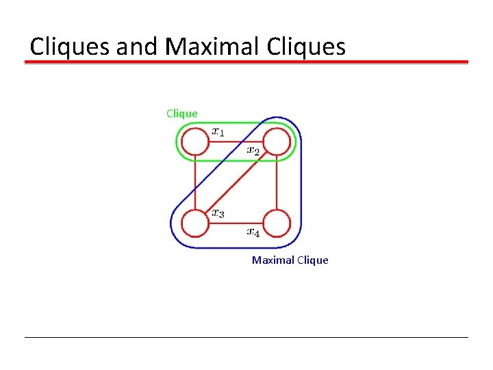
Cliques and Maximal Cliques Clique Maximal Clique

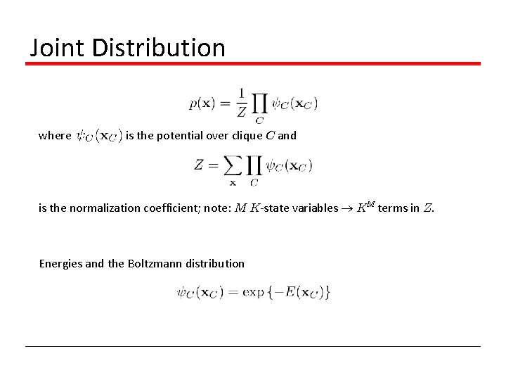
Joint Distribution where is the potential over clique C and is the normalization coefficient; note: M K-state variables KM terms in Z. Energies and the Boltzmann distribution

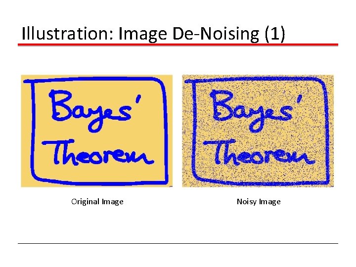
Illustration: Image De-Noising (1) Original Image Noisy Image

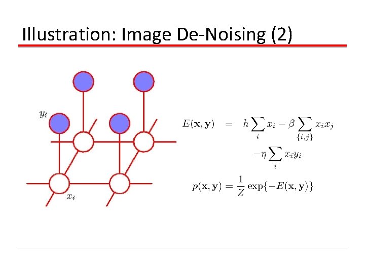
Illustration: Image De-Noising (2)

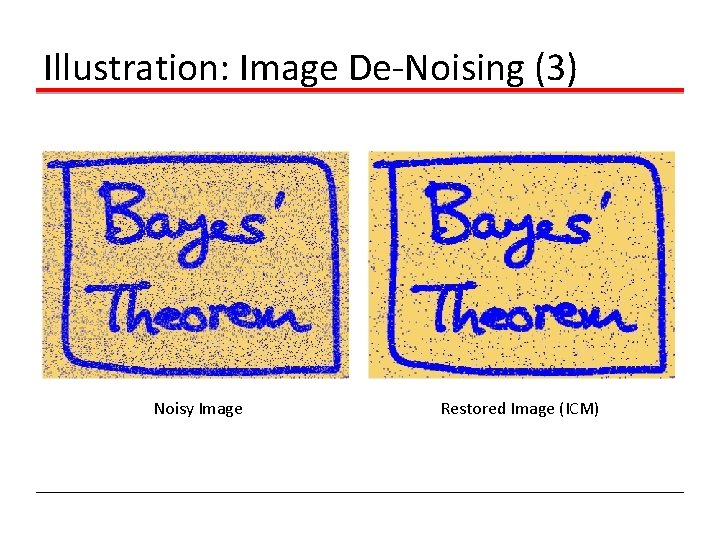
Illustration: Image De-Noising (3) Noisy Image Restored Image (ICM)

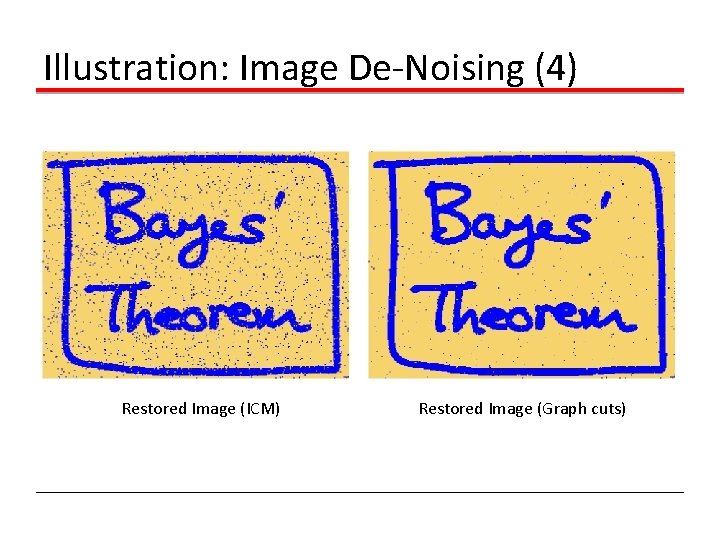
Illustration: Image De-Noising (4) Restored Image (ICM) Restored Image (Graph cuts)

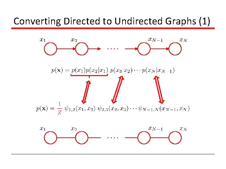
Converting Directed to Undirected Graphs (1)

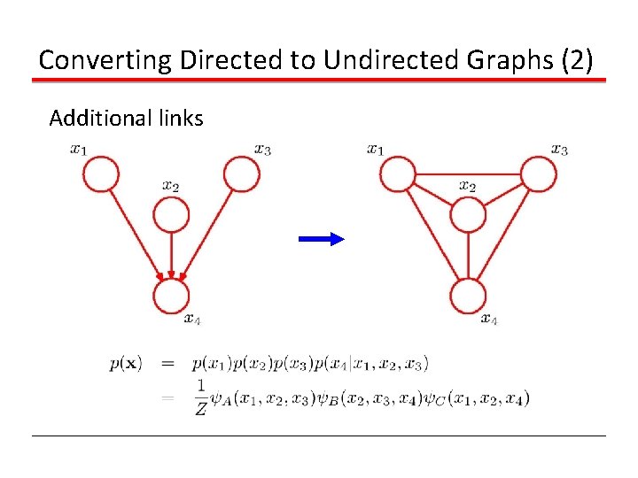
Converting Directed to Undirected Graphs (2) Additional links

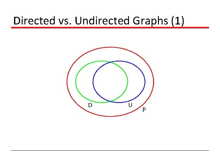
Directed vs. Undirected Graphs (1)

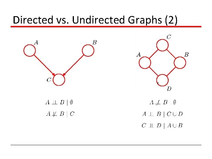
Directed vs. Undirected Graphs (2)

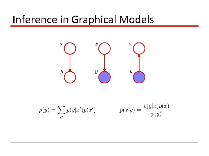
Inference in Graphical Models

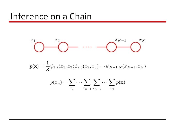
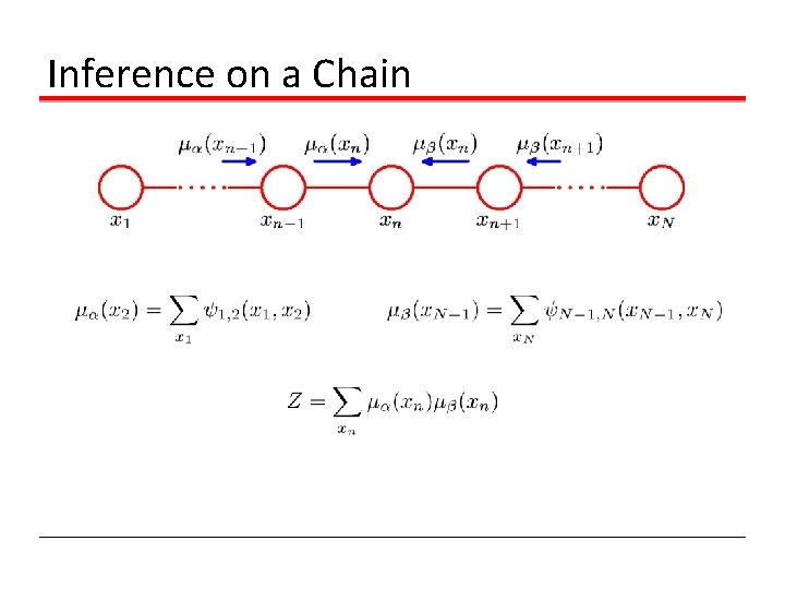
Inference on a Chain

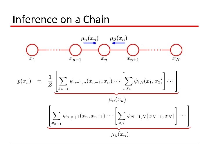
Inference on a Chain

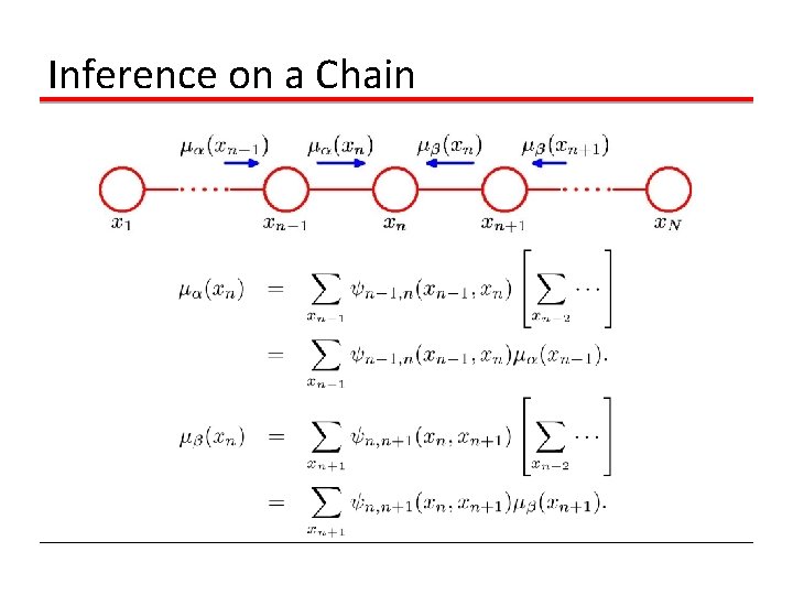
Inference on a Chain

Inference on a Chain

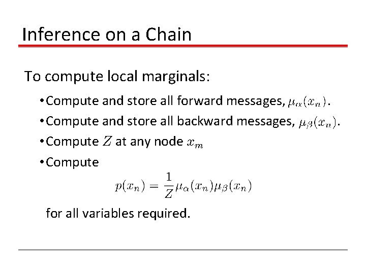
Inference on a Chain To compute local marginals: • Compute and store all forward messages, • Compute and store all backward messages, • Compute Z at any node xm • Compute for all variables required. . .

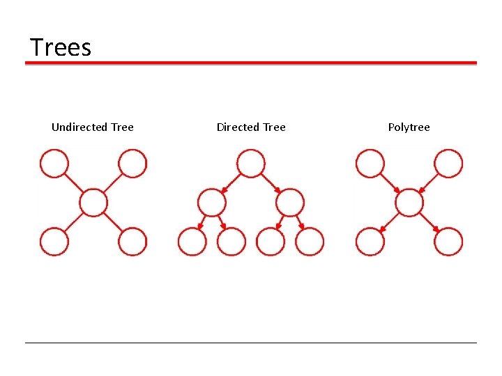
Trees Undirected Tree Directed Tree Polytree

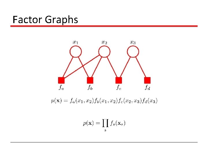
Factor Graphs

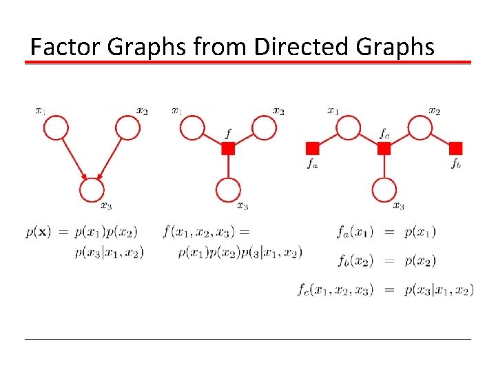
Factor Graphs from Directed Graphs

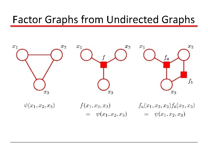
Factor Graphs from Undirected Graphs

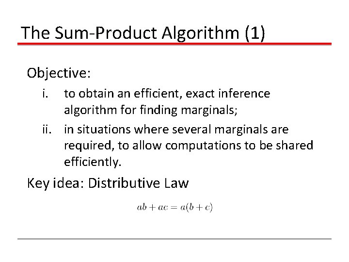
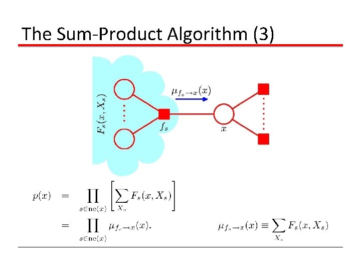
The Sum-Product Algorithm (1) Objective: i. to obtain an efficient, exact inference algorithm for finding marginals; ii. in situations where several marginals are required, to allow computations to be shared efficiently. Key idea: Distributive Law

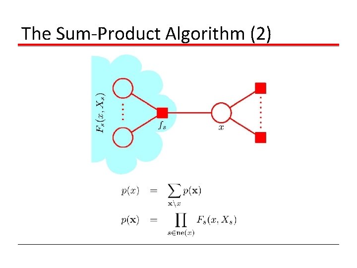
The Sum-Product Algorithm (2)

The Sum-Product Algorithm (3)

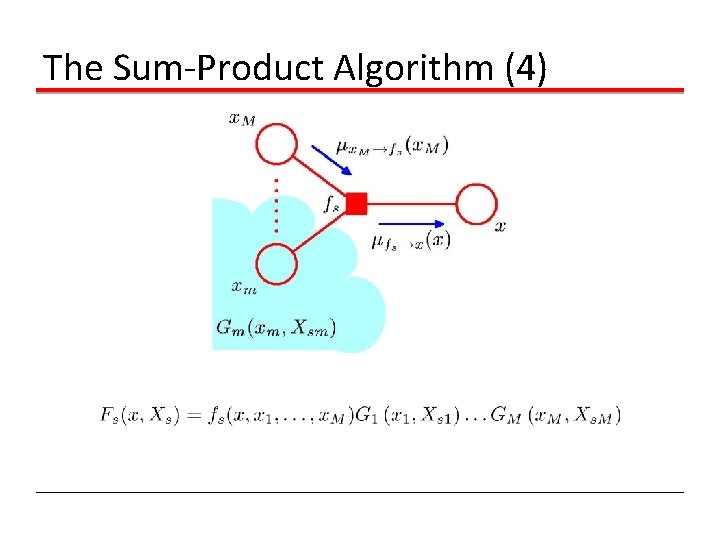
The Sum-Product Algorithm (4)

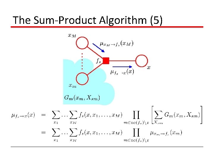
The Sum-Product Algorithm (5)

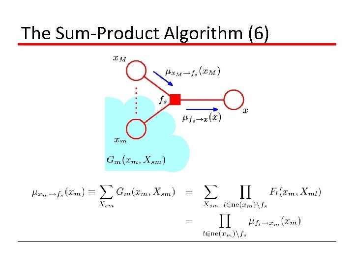
The Sum-Product Algorithm (6)

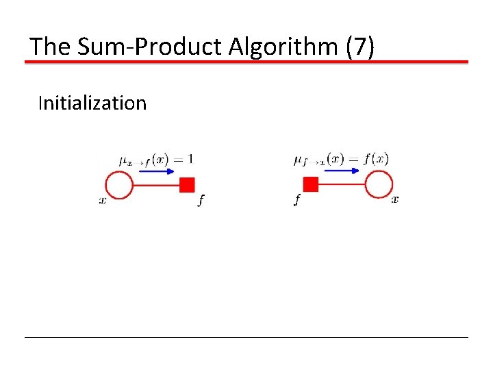
The Sum-Product Algorithm (7) Initialization

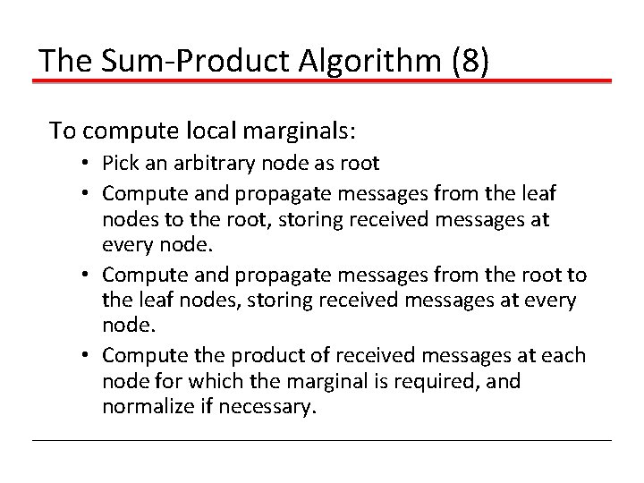
The Sum-Product Algorithm (8) To compute local marginals: • Pick an arbitrary node as root • Compute and propagate messages from the leaf nodes to the root, storing received messages at every node. • Compute and propagate messages from the root to the leaf nodes, storing received messages at every node. • Compute the product of received messages at each node for which the marginal is required, and normalize if necessary.

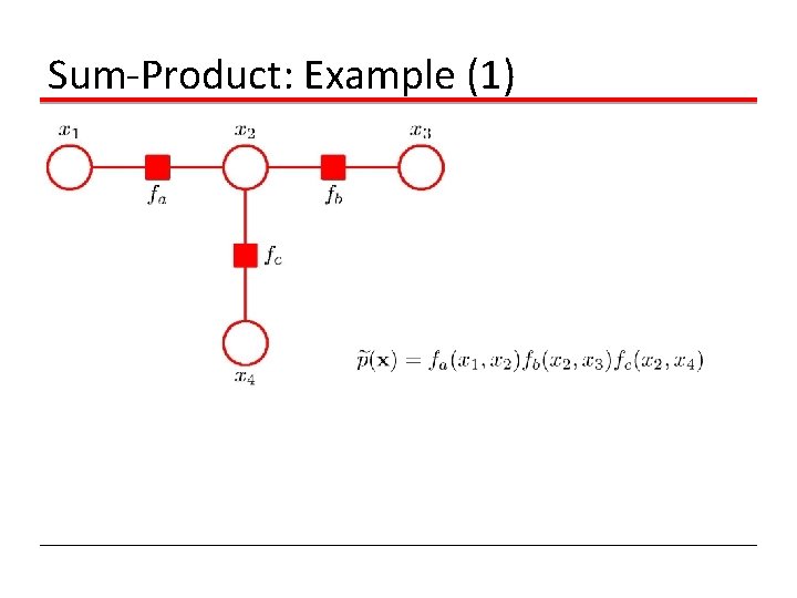
Sum-Product: Example (1)

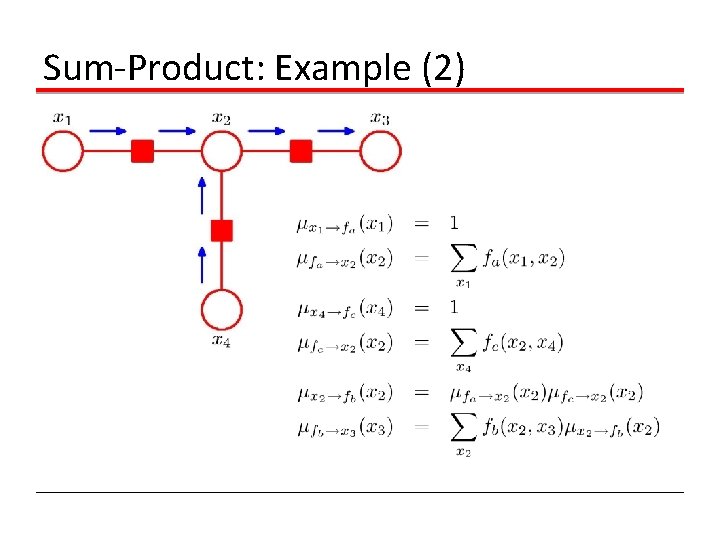
Sum-Product: Example (2)

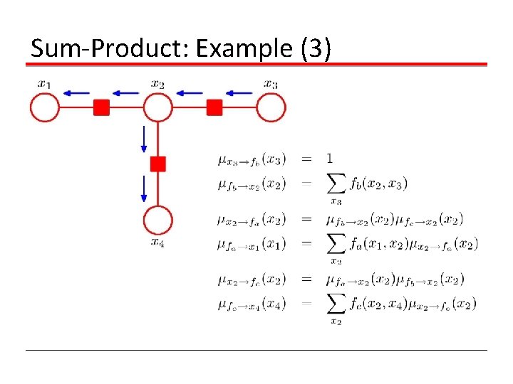
Sum-Product: Example (3)

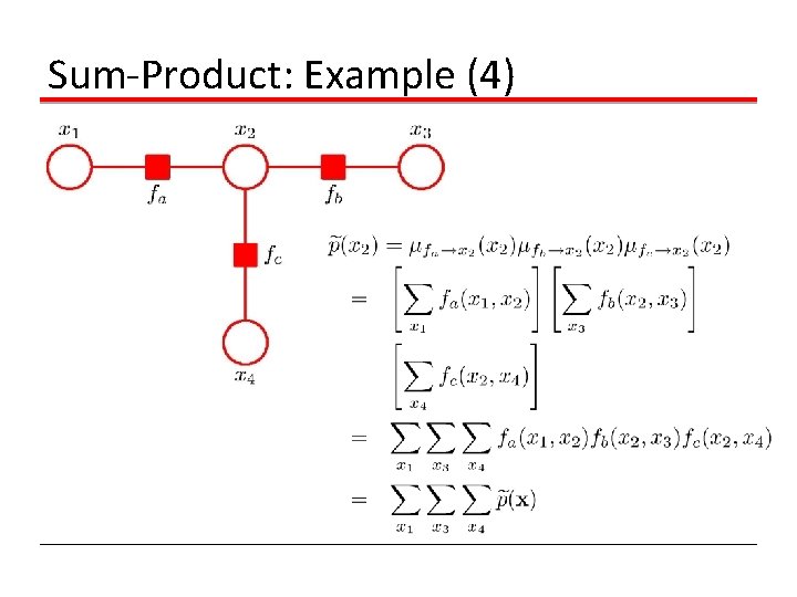
Sum-Product: Example (4)

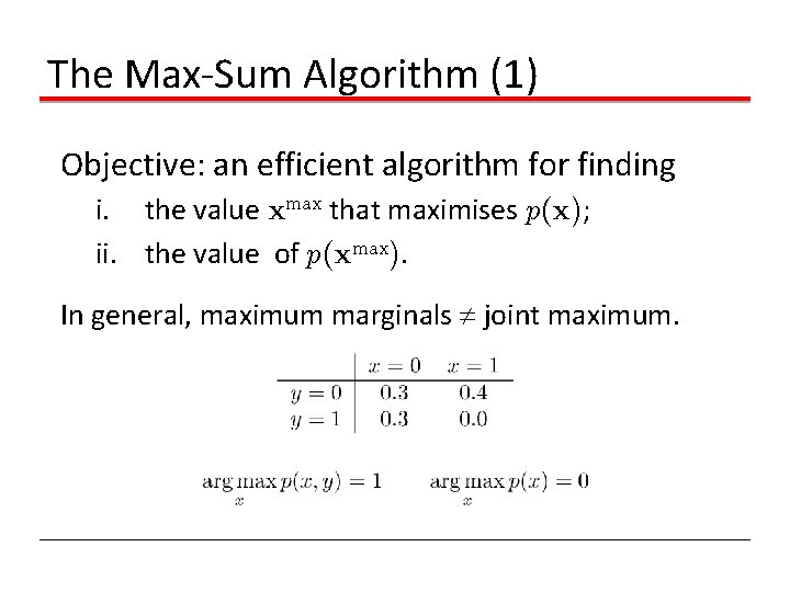
The Max-Sum Algorithm (1) Objective: an efficient algorithm for finding i. the value xmax that maximises p(x); ii. the value of p(xmax). In general, maximum marginals joint maximum.

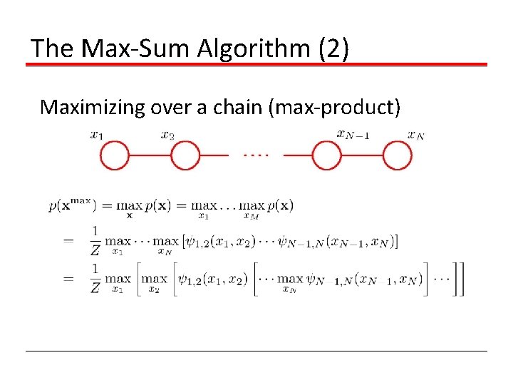
The Max-Sum Algorithm (2) Maximizing over a chain (max-product)

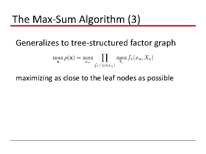
The Max-Sum Algorithm (3) Generalizes to tree-structured factor graph maximizing as close to the leaf nodes as possible

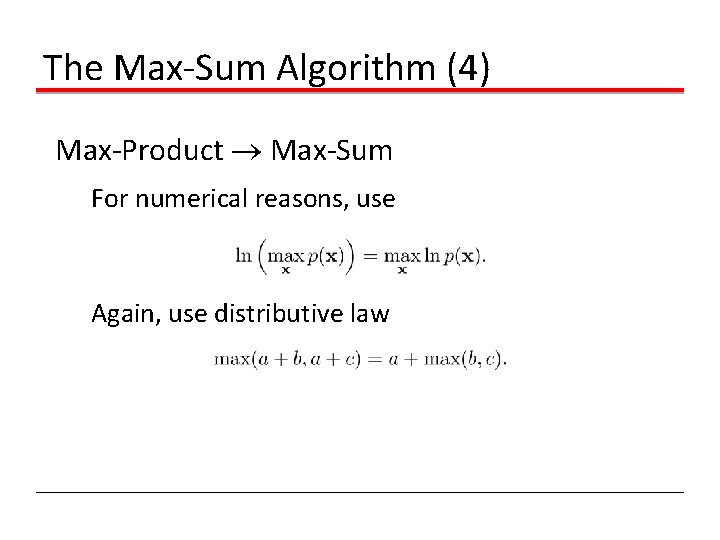
The Max-Sum Algorithm (4) Max-Product Max-Sum For numerical reasons, use Again, use distributive law

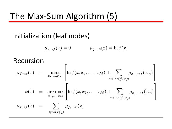
The Max-Sum Algorithm (5) Initialization (leaf nodes) Recursion

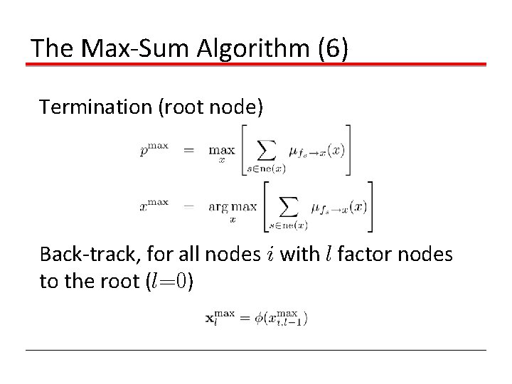
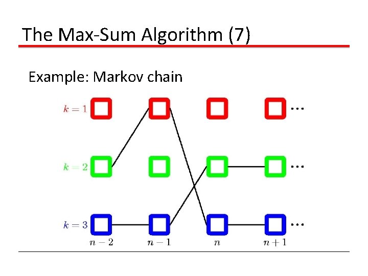
The Max-Sum Algorithm (6) Termination (root node) Back-track, for all nodes i with l factor nodes to the root (l=0)

The Max-Sum Algorithm (7) Example: Markov chain

The Junction Tree Algorithm • Exact inference on general graphs. • Works by turning the initial graph into a junction tree and then running a sumproduct-like algorithm. • Intractable on graphs with large cliques.

Loopy Belief Propagation • Sum-Product on general graphs. • Initial unit messages passed across all links, after which messages are passed around until convergence (not guaranteed!). • Approximate but tractable for large graphs. • Sometime works well, sometimes not at all.