Ch 8 Graphical Models Pattern Recognition and Machine

Ch 8. Graphical Models Pattern Recognition and Machine Learning, C. M. Bishop, 2006. Revised by M. -O. Heo Summarized by J. W. Nam Biointelligence Laboratory, Seoul National University http: //bi. snu. ac. kr/ 1

Contents l 8. 1 Bayesian network ¨ 8. 1. 1 Example of Bayesian network – polynomial regression ¨ 8. 1. 2 Generative models ¨ 8. 1. 3 Discrete variables ¨ 8. 1. 4 Linear Gaussian models l 8. 2 Conditional independence ¨ 8. 2. 1 Three example graphs ¨ 8. 2. 2 d-separation (C) 2007, SNU Biointelligence Lab, http: //bi. snu. ac. kr/ 2

Probability play a central role in modern pattern recognition l All of the probabilistic inference and learning amount to repeated application of the sum rule and the product rule l There are useful properties in using probabilistic graphical models l ¨ A simple way to visualize the structure of a probabilistic model ¨ Insights into the properties of the model ¨ Complex computations (for inference and learning) can be expressed in terms of graphical manipulations underlying mathematical expressions. (C) 2007, SNU Biointelligence Lab, http: //bi. snu. ac. kr/ 3

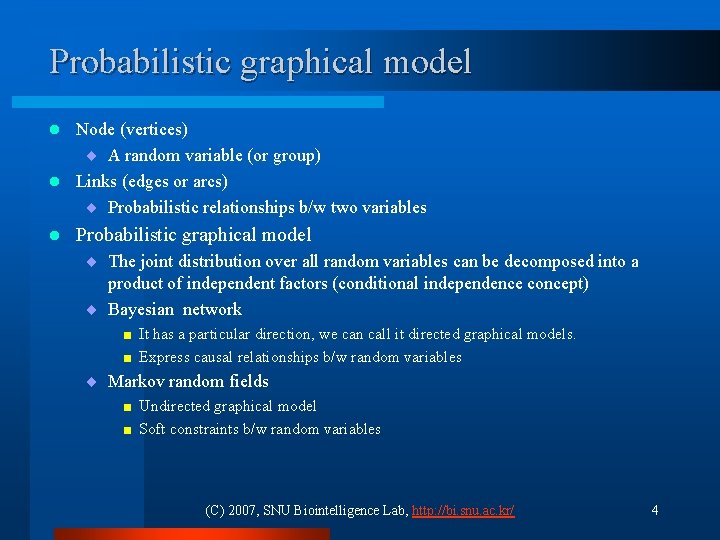
Probabilistic graphical model Node (vertices) ¨ A random variable (or group) l Links (edges or arcs) ¨ Probabilistic relationships b/w two variables l l Probabilistic graphical model ¨ The joint distribution over all random variables can be decomposed into a product of independent factors (conditional independence concept) ¨ Bayesian network < < It has a particular direction, we can call it directed graphical models. Express causal relationships b/w random variables ¨ Markov random fields < < Undirected graphical model Soft constraints b/w random variables (C) 2007, SNU Biointelligence Lab, http: //bi. snu. ac. kr/ 4

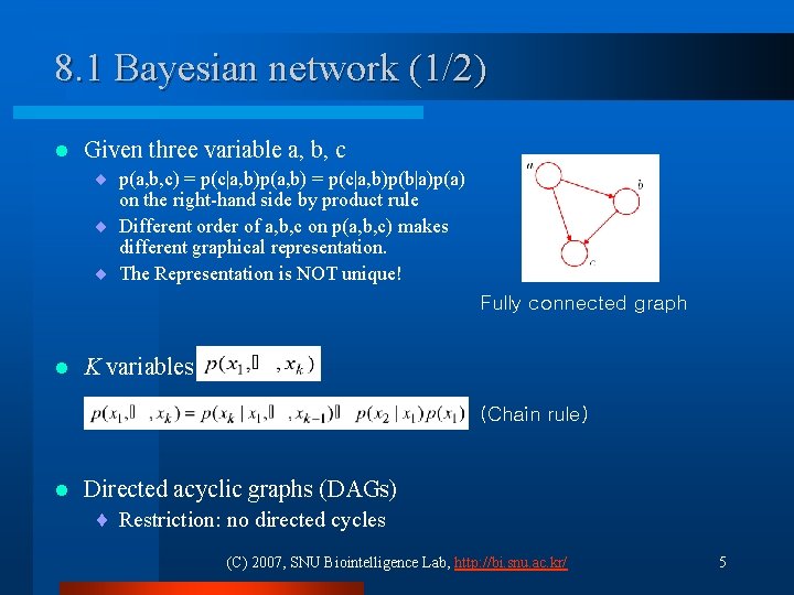
8. 1 Bayesian network (1/2) l Given three variable a, b, c ¨ p(a, b, c) = p(c|a, b)p(a, b) = p(c|a, b)p(b|a)p(a) on the right-hand side by product rule ¨ Different order of a, b, c on p(a, b, c) makes different graphical representation. ¨ The Representation is NOT unique! Fully connected graph l K variables (Chain rule) l Directed acyclic graphs (DAGs) ¨ Restriction: no directed cycles (C) 2007, SNU Biointelligence Lab, http: //bi. snu. ac. kr/ 5

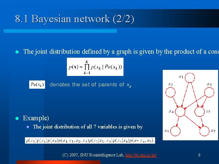
8. 1 Bayesian network (2/2) l The joint distribution defined by a graph is given by the product of a cond denotes the set of parents of xk l Example) ¨ The joint distribution of all 7 variables is given by (C) 2007, SNU Biointelligence Lab, http: //bi. snu. ac. kr/ 6

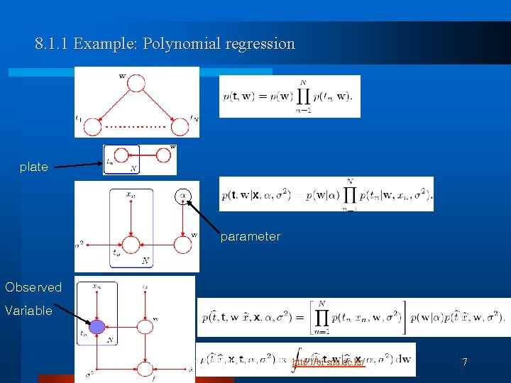
8. 1. 1 Example: Polynomial regression plate parameter Observed Variable (C) 2007, SNU Biointelligence Lab, http: //bi. snu. ac. kr/ 7

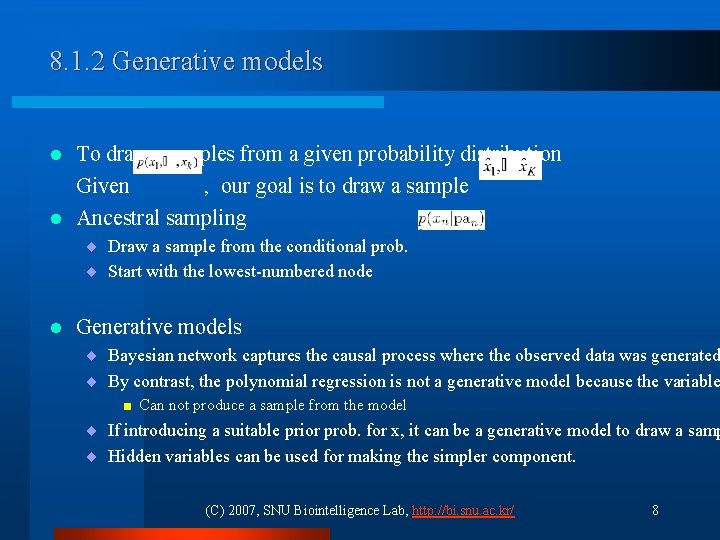
8. 1. 2 Generative models To draws samples from a given probability distribution Given , our goal is to draw a sample l Ancestral sampling l ¨ Draw a sample from the conditional prob. ¨ Start with the lowest-numbered node l Generative models ¨ Bayesian network captures the causal process where the observed data was generated ¨ By contrast, the polynomial regression is not a generative model because the variable < Can not produce a sample from the model ¨ If introducing a suitable prior prob. for x, it can be a generative model to draw a samp ¨ Hidden variables can be used for making the simpler component. (C) 2007, SNU Biointelligence Lab, http: //bi. snu. ac. kr/ 8

Nodes as building blocks in Graphical models l The framework of graphical models is very useful in expressing the way in which “building blocks” are linked together. l Choose the relationship b/w each parent-child pair in a directed graph to be conjugate. ¨ The followings can extend hierarchically to construct arbitrarily complex DAGs. < < Discrete variables Gaussian variables (C) 2007, SNU Biointelligence Lab, http: //bi. snu. ac. kr/ 9

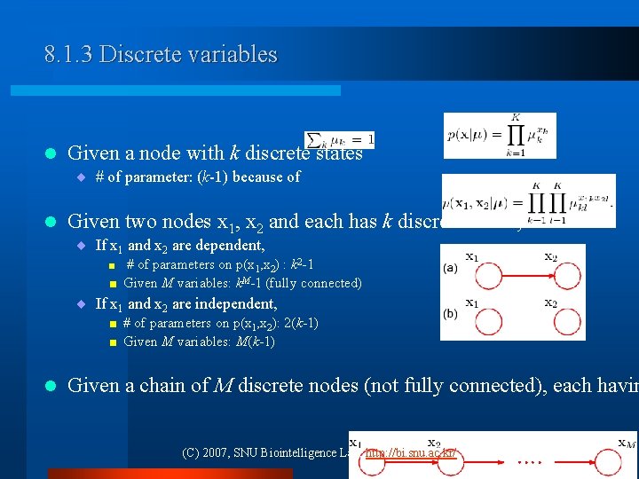
8. 1. 3 Discrete variables l Given a node with k discrete states ¨ # of parameter: (k-1) because of l Given two nodes x 1, x 2 and each has k discrete states, ¨ If x 1 and x 2 are dependent, < < # of parameters on p(x 1, x 2) : k 2 -1 Given M variables: k. M-1 (fully connected) ¨ If x 1 and x 2 are independent, < < l # of parameters on p(x 1, x 2): 2(k-1) Given M variables: M(k-1) Given a chain of M discrete nodes (not fully connected), each havin (C) 2007, SNU Biointelligence Lab, http: //bi. snu. ac. kr/ 10

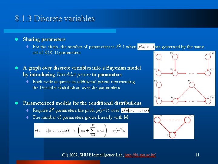
8. 1. 3 Discrete variables l Sharing parameters ¨ For the chain, the number of parameters is K 2 -1 when set of K(K-1) parameters l are governed by the same A graph over discrete variables into a Bayesian model by introducing Dirichlet priors to parameters ¨ Each node acquires an additional parent representing the Dirichlet distribution over the parameters l Parameterized models for the conditional distributions ¨ Require 2 M parameters the prob. p(y=1) over ¨ The number of parameters grows linearly with M (C) 2007, SNU Biointelligence Lab, http: //bi. snu. ac. kr/ 11

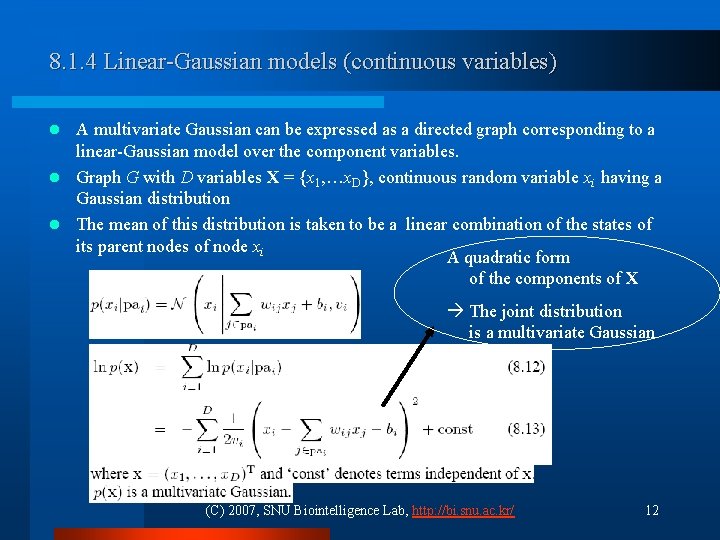
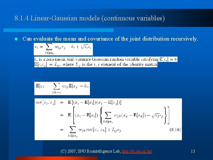
8. 1. 4 Linear-Gaussian models (continuous variables) A multivariate Gaussian can be expressed as a directed graph corresponding to a linear-Gaussian model over the component variables. l Graph G with D variables X = {x 1, …x. D}, continuous random variable xi having a Gaussian distribution l The mean of this distribution is taken to be a linear combination of the states of its parent nodes of node xi A quadratic form of the components of X l The joint distribution is a multivariate Gaussian (C) 2007, SNU Biointelligence Lab, http: //bi. snu. ac. kr/ 12

8. 1. 4 Linear-Gaussian models (continuous variables) l Can evaluate the mean and covariance of the joint distribution recursively. (C) 2007, SNU Biointelligence Lab, http: //bi. snu. ac. kr/ 13

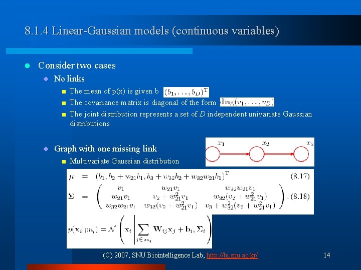
8. 1. 4 Linear-Gaussian models (continuous variables) l Consider two cases ¨ No links < < < The mean of p(x) is given b The covariance matrix is diagonal of the form The joint distribution represents a set of D independent univariate Gaussian distributions ¨ Graph with one missing link < Multivariate Gaussian distribution (C) 2007, SNU Biointelligence Lab, http: //bi. snu. ac. kr/ 14

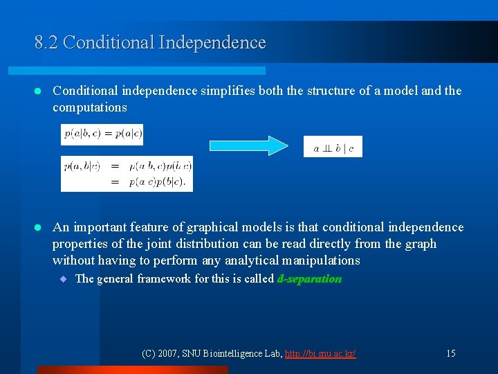
8. 2 Conditional Independence l Conditional independence simplifies both the structure of a model and the computations l An important feature of graphical models is that conditional independence properties of the joint distribution can be read directly from the graph without having to perform any analytical manipulations ¨ The general framework for this is called d-separation (C) 2007, SNU Biointelligence Lab, http: //bi. snu. ac. kr/ 15

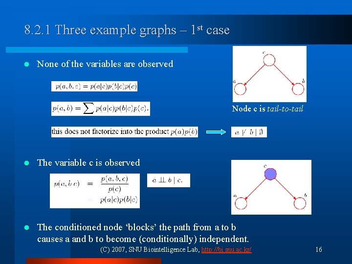
8. 2. 1 Three example graphs – 1 st case l None of the variables are observed Node c is tail-to-tail l The variable c is observed l The conditioned node ‘blocks’ the path from a to b causes a and b to become (conditionally) independent. (C) 2007, SNU Biointelligence Lab, http: //bi. snu. ac. kr/ 16

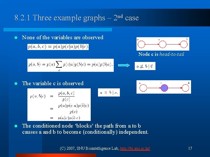
8. 2. 1 Three example graphs – 2 nd case l None of the variables are observed Node c is head-to-tail l The variable c is observed l The conditioned node ‘blocks’ the path from a to b causes a and b to become (conditionally) independent. (C) 2007, SNU Biointelligence Lab, http: //bi. snu. ac. kr/ 17

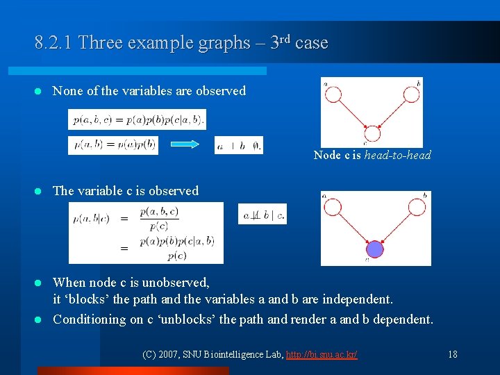
8. 2. 1 Three example graphs – 3 rd case l None of the variables are observed Node c is head-to-head l The variable c is observed When node c is unobserved, it ‘blocks’ the path and the variables a and b are independent. l Conditioning on c ‘unblocks’ the path and render a and b dependent. l (C) 2007, SNU Biointelligence Lab, http: //bi. snu. ac. kr/ 18

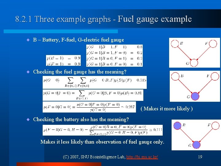
8. 2. 1 Three example graphs - Fuel gauge example ¨ B – Battery, F-fuel, G-electric fuel gauge ¨ Checking the fuel gauge has the meaning? ( Makes it more likely ) ¨ Checking the battery also has the meaning? Makes it less likely than observation of fuel gauge only. (C) 2007, SNU Biointelligence Lab, http: //bi. snu. ac. kr/ 19

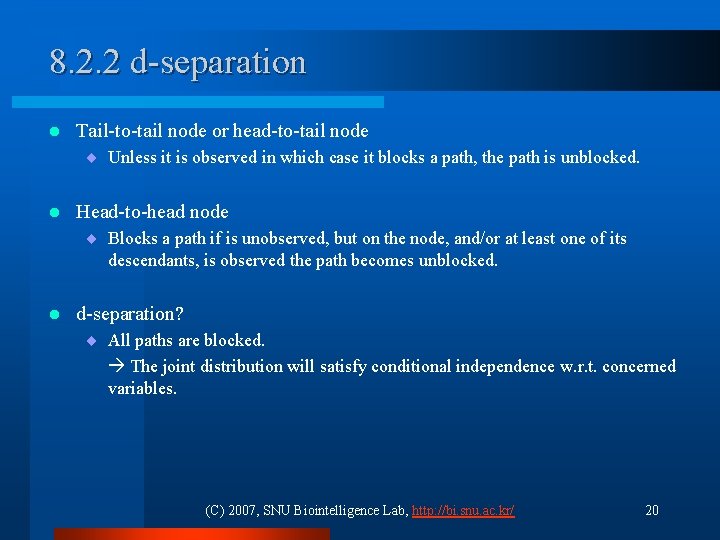
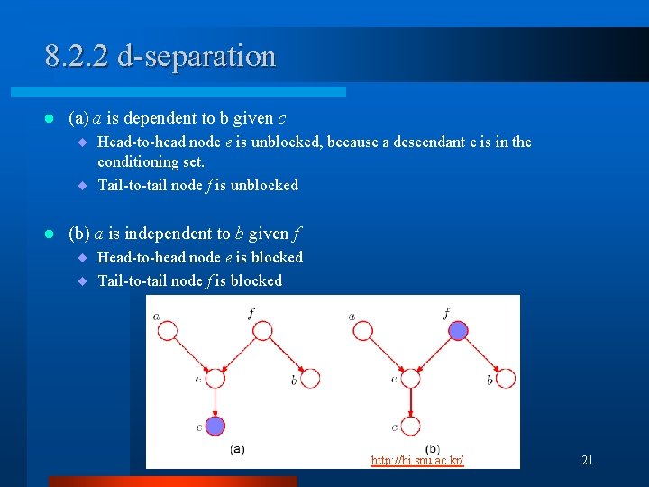
8. 2. 2 d-separation l Tail-to-tail node or head-to-tail node ¨ Unless it is observed in which case it blocks a path, the path is unblocked. l Head-to-head node ¨ Blocks a path if is unobserved, but on the node, and/or at least one of its descendants, is observed the path becomes unblocked. l d-separation? ¨ All paths are blocked. The joint distribution will satisfy conditional independence w. r. t. concerned variables. (C) 2007, SNU Biointelligence Lab, http: //bi. snu. ac. kr/ 20

8. 2. 2 d-separation l (a) a is dependent to b given c ¨ Head-to-head node e is unblocked, because a descendant c is in the conditioning set. ¨ Tail-to-tail node f is unblocked l (b) a is independent to b given f ¨ Head-to-head node e is blocked ¨ Tail-to-tail node f is blocked (C) 2007, SNU Biointelligence Lab, http: //bi. snu. ac. kr/ 21

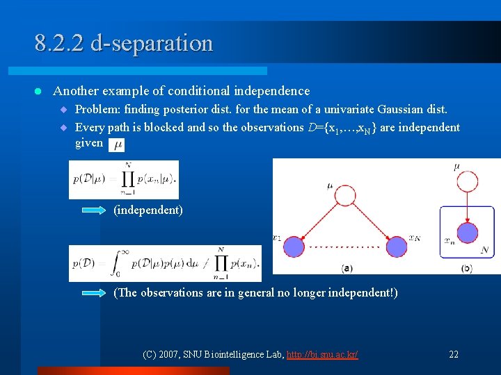
8. 2. 2 d-separation l Another example of conditional independence ¨ Problem: finding posterior dist. for the mean of a univariate Gaussian dist. ¨ Every path is blocked and so the observations D={x 1, …, x. N} are independent given (independent) (The observations are in general no longer independent!) (C) 2007, SNU Biointelligence Lab, http: //bi. snu. ac. kr/ 22

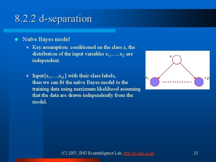
8. 2. 2 d-separation l Naïve Bayes model ¨ Key assumption: conditioned on the class z, the distribution of the input variables x 1, …, x. D are independent. ¨ Input{x 1, …, x. N} with their class labels, then we can fit the naïve Bayes model to the training data using maximum likelihood assuming that the data are drawn independently from the model. (C) 2007, SNU Biointelligence Lab, http: //bi. snu. ac. kr/ 23

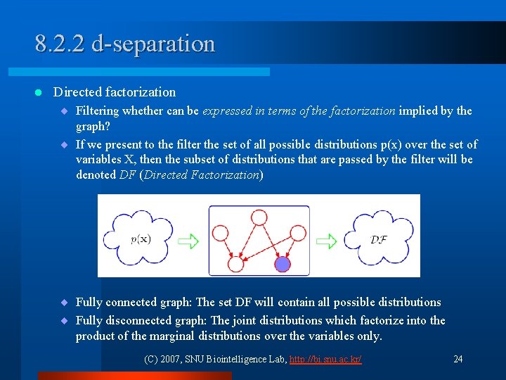
8. 2. 2 d-separation l Directed factorization ¨ Filtering whether can be expressed in terms of the factorization implied by the graph? ¨ If we present to the filter the set of all possible distributions p(x) over the set of variables X, then the subset of distributions that are passed by the filter will be denoted DF (Directed Factorization) ¨ Fully connected graph: The set DF will contain all possible distributions ¨ Fully disconnected graph: The joint distributions which factorize into the product of the marginal distributions over the variables only. (C) 2007, SNU Biointelligence Lab, http: //bi. snu. ac. kr/ 24

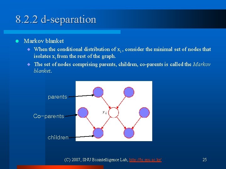
8. 2. 2 d-separation l Markov blanket ¨ When the conditional distribution of xi , consider the minimal set of nodes that isolates xi from the rest of the graph. ¨ The set of nodes comprising parents, children, co-parents is called the Markov blanket. parents Co-parents children (C) 2007, SNU Biointelligence Lab, http: //bi. snu. ac. kr/ 25