Deep Learning Tutorial Courtesy of Hungyi Lee Machine

Deep Learning Tutorial Courtesy of Hung-yi Lee

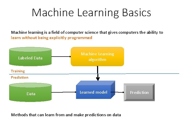
Machine Learning Basics Machine learning is a field of computer science that gives computers the ability to learn without being explicitly programmed Labeled Data Machine Learning algorithm Training Prediction Data Learned model Methods that can learn from and make predictions on data Prediction

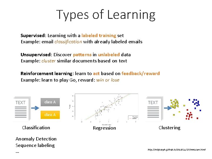
Types of Learning Supervised: Learning with a labeled training set Example: email classification with already labeled emails Unsupervised: Discover patterns in unlabeled data Example: cluster similar documents based on text Reinforcement learning: learn to act based on feedback/reward Example: learn to play Go, reward: win or lose class A Classification Anomaly Detection Sequence labeling … Regression Clustering http: //mbjoseph. github. io/2013/11/27/measure. html

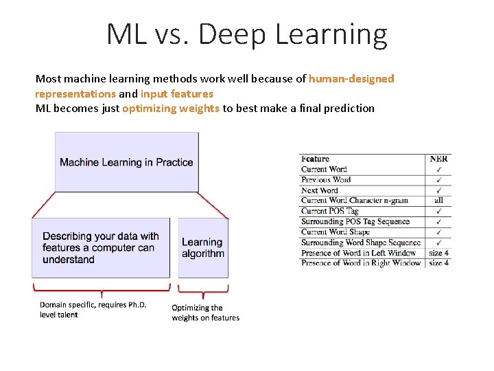
ML vs. Deep Learning Most machine learning methods work well because of human-designed representations and input features ML becomes just optimizing weights to best make a final prediction

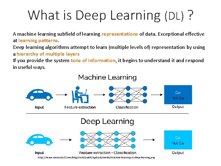
What is Deep Learning (DL) ? A machine learning subfield of learning representations of data. Exceptional effective at learning patterns. Deep learning algorithms attempt to learn (multiple levels of) representation by using a hierarchy of multiple layers If you provide the system tons of information, it begins to understand it and respond in useful ways. https: //www. xenonstack. com/blog/static/public/uploads/media/machine-learning-vs-deep-learning. png

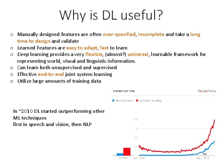
Why is DL useful? o Manually designed features are often over-specified, incomplete and take a long time to design and validate o Learned Features are easy to adapt, fast to learn o Deep learning provides a very flexible, (almost? ) universal, learnable framework for representing world, visual and linguistic information. o Can learn both unsupervised and supervised o Effective end-to-end joint system learning o Utilize large amounts of training data In ~2010 DL started outperforming other ML techniques first in speech and vision, then NLP

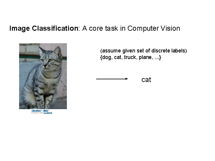
Image Classification: A core task in Computer Vision (assume given set of discrete labels) {dog, cat, truck, plane, . . . } cat This image by Nikita is licensed under CC-BY 2. 0 Lecture 2 - 7

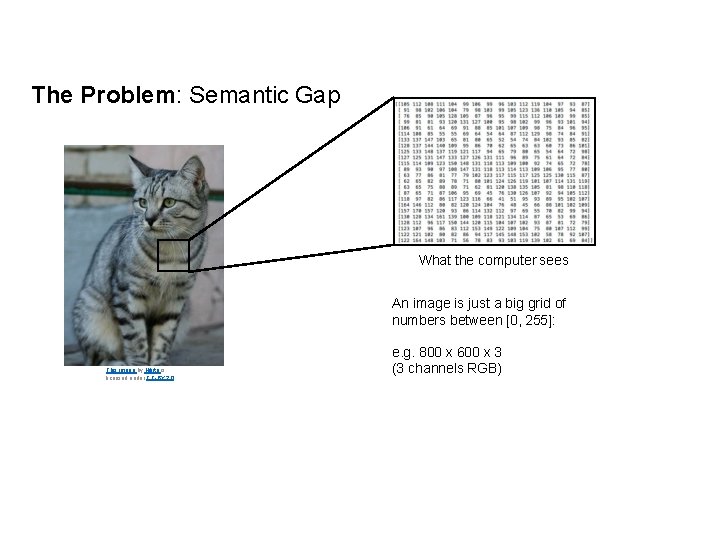
The Problem: Semantic Gap What the computer sees An image is just a big grid of numbers between [0, 255]: This image by Nikita is licensed under CC-BY 2. 0 e. g. 800 x 600 x 3 (3 channels RGB) Lecture 2 - 8

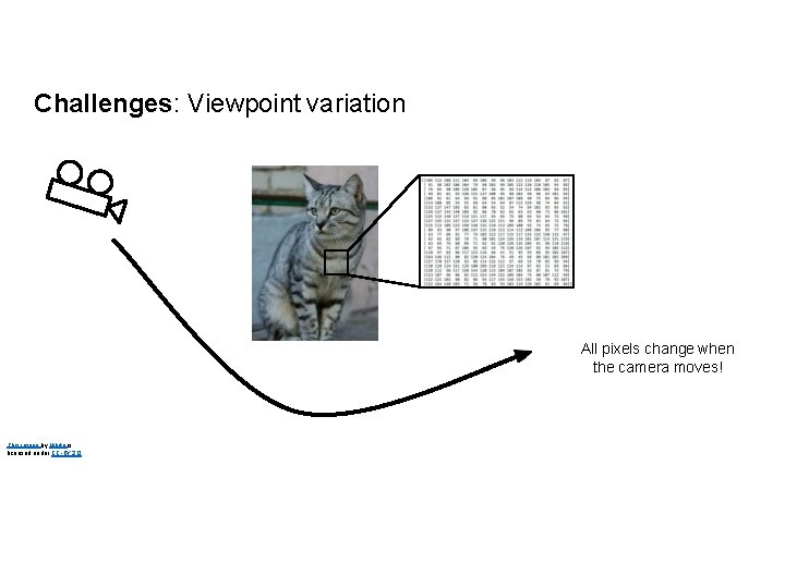
Challenges: Viewpoint variation All pixels change when the camera moves! This image by Nikita is licensed under CC-BY 2. 0 Lecture 2 - 9

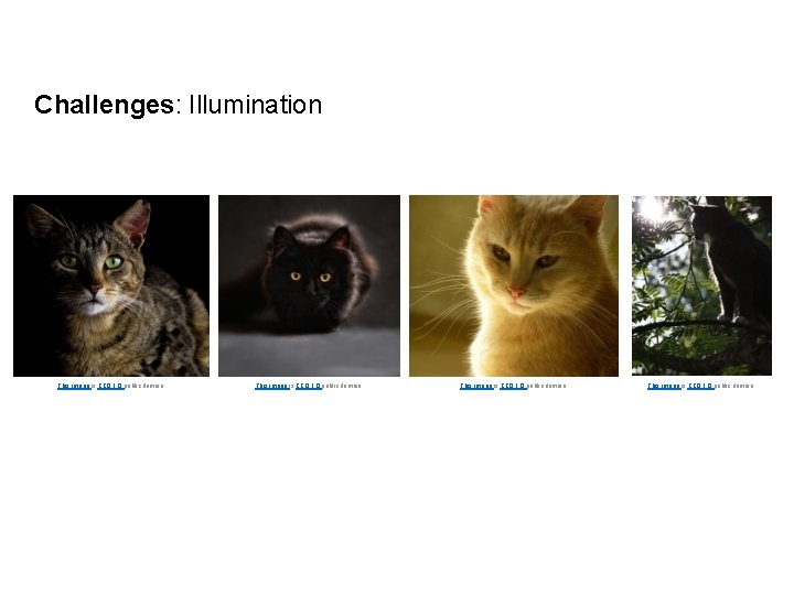
Challenges: Illumination This image is CC 0 1. 0 public domain Lecture 2 - This image is CC 0 1. 0 public domain

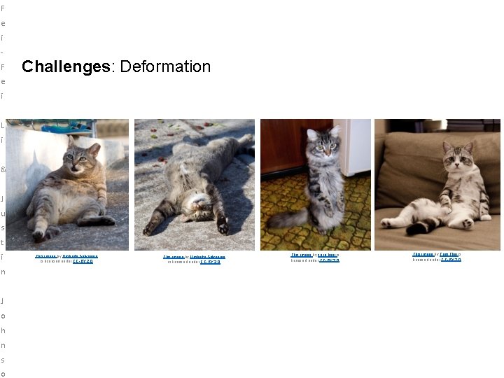
F e i F Challenges: Deformation e i L i & J u s t i This image by Umberto Salvagnin is licensed under CC-BY 2. 0 This image by sare bear is licensed under CC-BY 2. 0 n J o h n s o Lecture 2 - This image by Tom Thai is licensed under CC-BY 2. 0

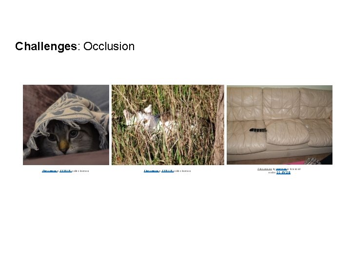
Challenges: Occlusion This image is CC 0 1. 0 public domain This image by jonsson is licensed under CC-BY 2. 0 This image is CC 0 1. 0 public domain Lecture 2 -

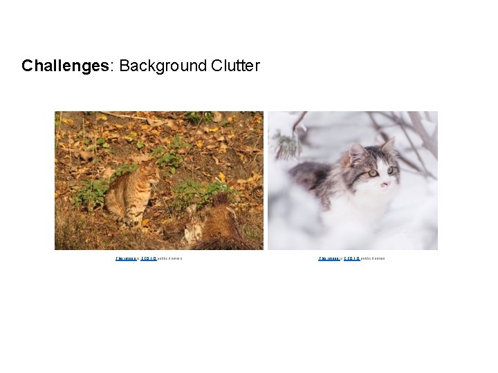
Challenges: Background Clutter This image is CC 0 1. 0 public domain Lecture 2 -

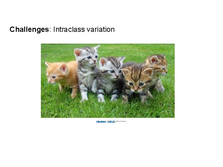
Challenges: Intraclass variation This image is CC 0 1. 0 public domain Lecture 2 -

Linear Classification Lecture 2 -

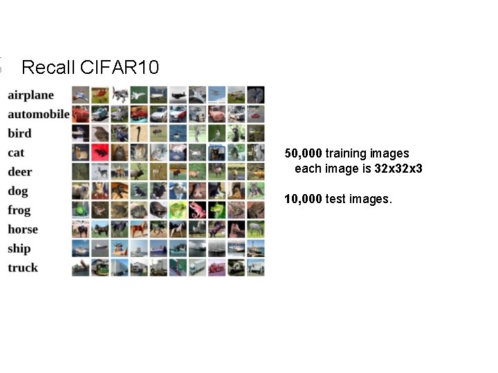
1 8 Recall CIFAR 10 50, 000 training images each image is 32 x 3 10, 000 test images. Lecture 2 -

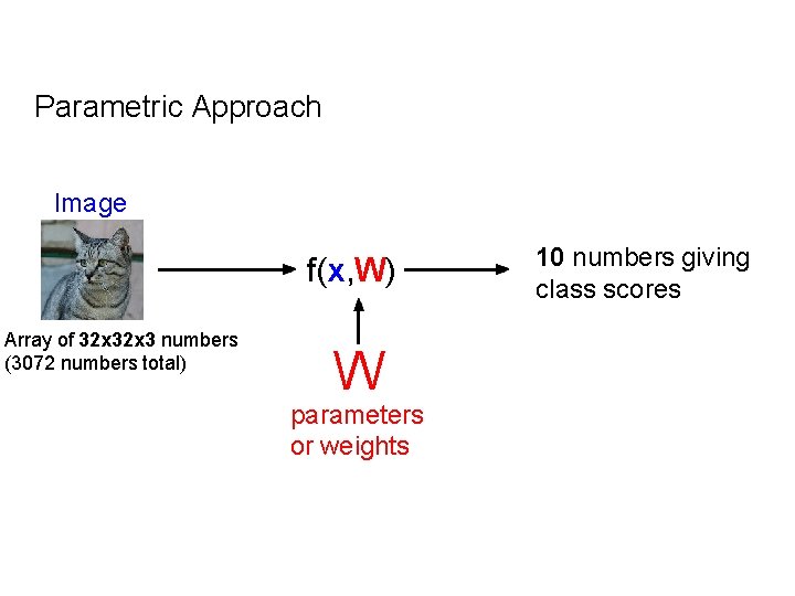
Parametric Approach Image f(x, W) Array of 32 x 3 numbers (3072 numbers total) 10 numbers giving class scores W parameters or weights Lecture 2 -

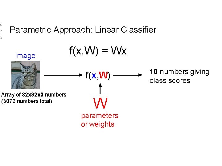
0 u 1 n Parametric Approach: Linear Classifier 8 g Image f(x, W) = Wx f(x, W) Array of 32 x 3 numbers (3072 numbers total) 10 numbers giving class scores W parameters or weights Lecture 2 -

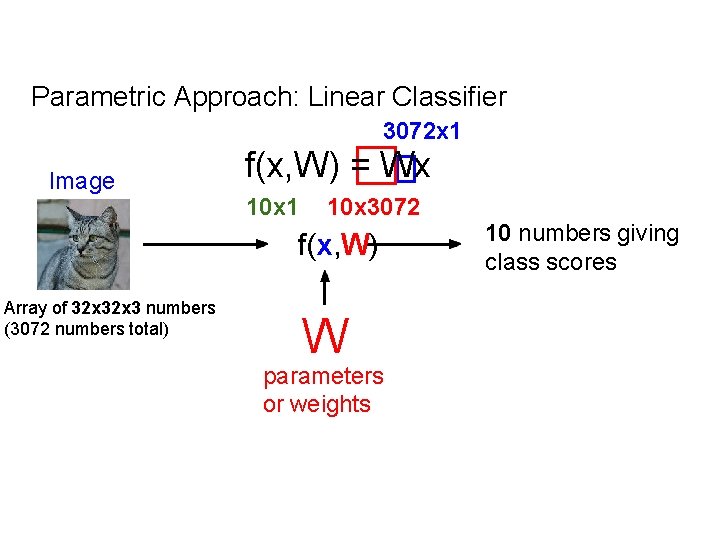
Parametric Approach: Linear Classifier 3072 x 1 Image f(x, W) = Wx 10 x 1 10 x 3072 f(x, W) Array of 32 x 3 numbers (3072 numbers total) 10 numbers giving class scores W parameters or weights Lecture 2 -

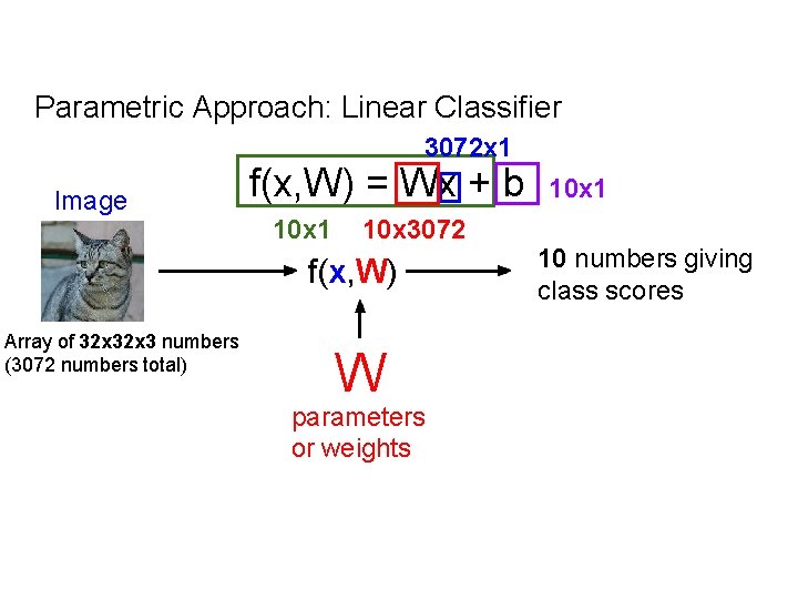
Parametric Approach: Linear Classifier 3072 x 1 Image f(x, W) = Wx + b 10 x 1 10 x 3072 f(x, W) Array of 32 x 3 numbers (3072 numbers total) 10 x 1 10 numbers giving class scores W parameters or weights Lecture 2 -

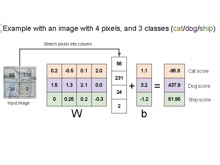
n g Example with an image with 4 pixels, and 3 classes (cat/dog/ship) Stretch pixels into column 56 56 24 231 2 Input image 0. 2 -0. 5 0. 1 2. 0 1. 1 231 1. 5 1. 3 2. 1 0. 0 24 0 0. 25 0. 2 W -0. 3 + 3. 2 -1. 2 2 b Lecture 2 - = -96. 8 Cat score 437. 9 Dog score 61. 95 Ship score

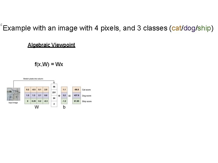
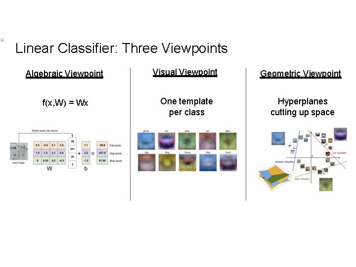
g Example with an image with 4 pixels, and 3 classes (cat/dog/ship) Algebraic Viewpoint f(x, W) = Wx Lecture 2 -

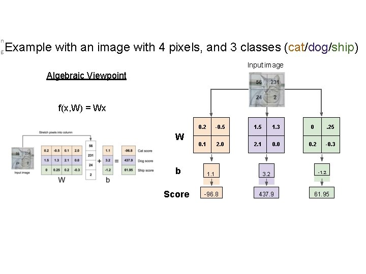
n g Example with an image with 4 pixels, and 3 classes (cat/dog/ship) Input image Algebraic Viewpoint f(x, W) = Wx W b Score 0. 2 -0. 5 1. 3 0 . 25 0. 1 2. 0 2. 1 0. 0 0. 2 -0. 3 1. 1 3. 2 -1. 2 -96. 8 437. 9 61. 95 Lecture 2 -

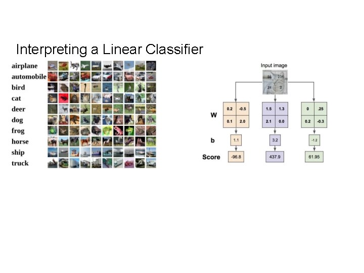
Interpreting a Linear Classifier Lecture 2 -

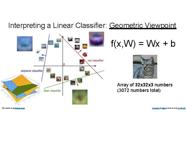
Interpreting a Linear Classifier: Geometric Viewpoint f(x, W) = Wx + b Array of 32 x 3 numbers (3072 numbers total) Plot created using Wolfram Cloud Cat image by Nikita is licensed under CC-BY 2. 0 Lecture 2 -

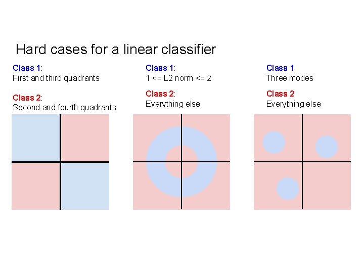
Hard cases for a linear classifier Class 1: First and third quadrants Class 1: 1 <= L 2 norm <= 2 Class 1: Three modes Class 2: Second and fourth quadrants Class 2: Everything else Lecture 2 -

u Linear Classifier: Three Viewpoints Algebraic Viewpoint Visual Viewpoint Geometric Viewpoint f(x, W) = Wx One template per class Hyperplanes cutting up space Lecture 2 -

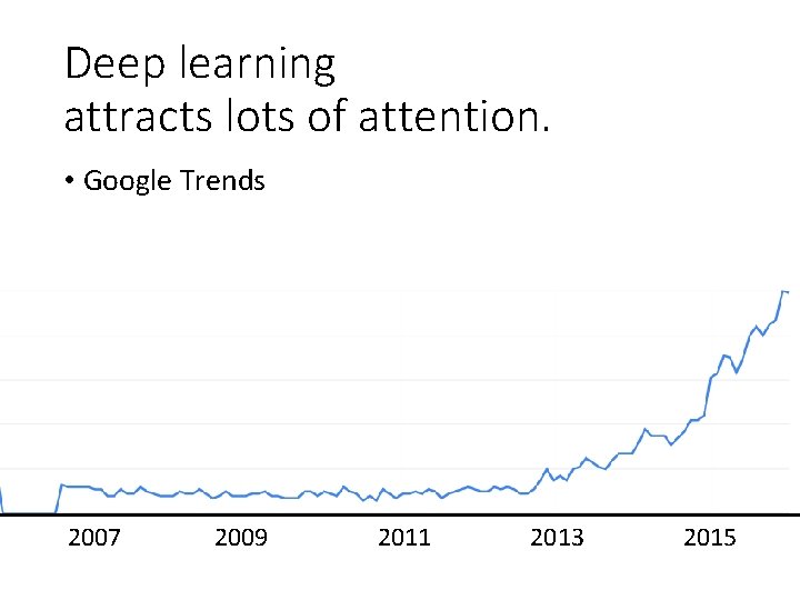
Deep learning attracts lots of attention. • Google Trends 2007 2009 2011 2013 2015

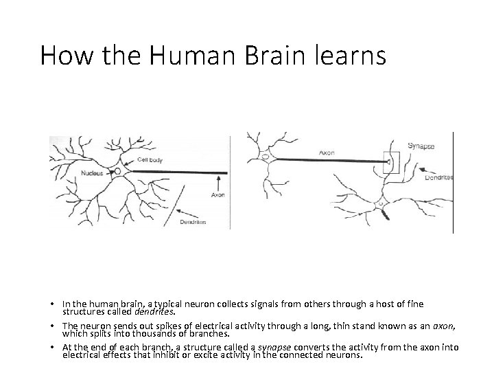
How the Human Brain learns • In the human brain, a typical neuron collects signals from others through a host of fine structures called dendrites. • The neuron sends out spikes of electrical activity through a long, thin stand known as an axon, which splits into thousands of branches. • At the end of each branch, a structure called a synapse converts the activity from the axon into electrical effects that inhibit or excite activity in the connected neurons.

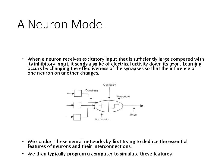
A Neuron Model • When a neuron receives excitatory input that is sufficiently large compared with its inhibitory input, it sends a spike of electrical activity down its axon. Learning occurs by changing the effectiveness of the synapses so that the influence of one neuron on another changes. • We conduct these neural networks by first trying to deduce the essential features of neurons and their interconnections. • We then typically program a computer to simulate these features.

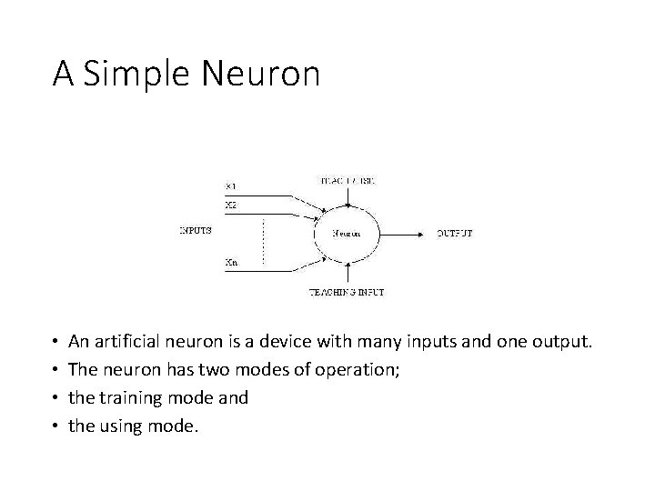
A Simple Neuron • • An artificial neuron is a device with many inputs and one output. The neuron has two modes of operation; the training mode and the using mode.

A Simple Neuron (Cont. ) • In the training mode, the neuron can be trained to fire (or not), for particular input patterns. • In the using mode, when a taught input pattern is detected at the input, its associated output becomes the current output. If the input pattern does not belong in the taught list of input patterns, the firing rule is used to determine whether to fire or not. • The firing rule is an important concept in neural networks and accounts for their high flexibility. A firing rule determines how one calculates whether a neuron should fire for any input pattern. It relates to all the input patterns, not only the ones on which the node was trained on previously.

Part I: Introduction of Deep Learning What people already knew in 1980 s

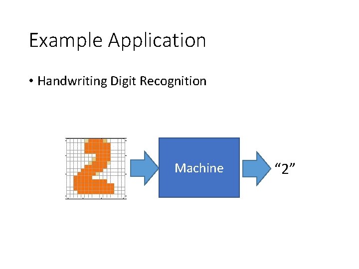
Example Application • Handwriting Digit Recognition Machine “ 2”

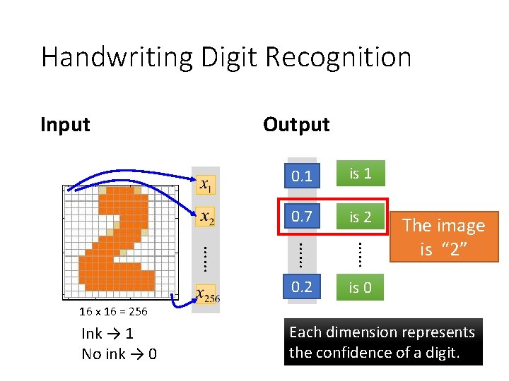
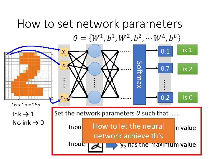
Handwriting Digit Recognition Input Output y 1 0. 1 is 1 0. 7 y 2 is 2 …… …… …… 0. 2 y 10 The image is “ 2” is 0 16 x 16 = 256 Ink → 1 No ink → 0 Each dimension represents the confidence of a digit.

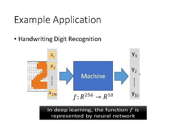
Example Application • Handwriting Digit Recognition y 1 “ 2” …… …… Machine y 2 y 10

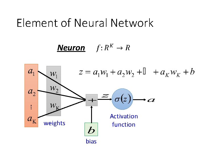
Element of Neural Network Neuron … Activation function weights bias

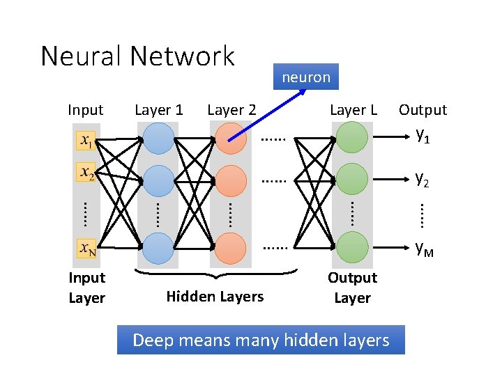
Neural Network Input Layer 1 neuron Layer 2 Layer L …… y 1 …… y 2 Hidden Layers …… …… …… Input Layer Output y. M Output Layer Deep means many hidden layers

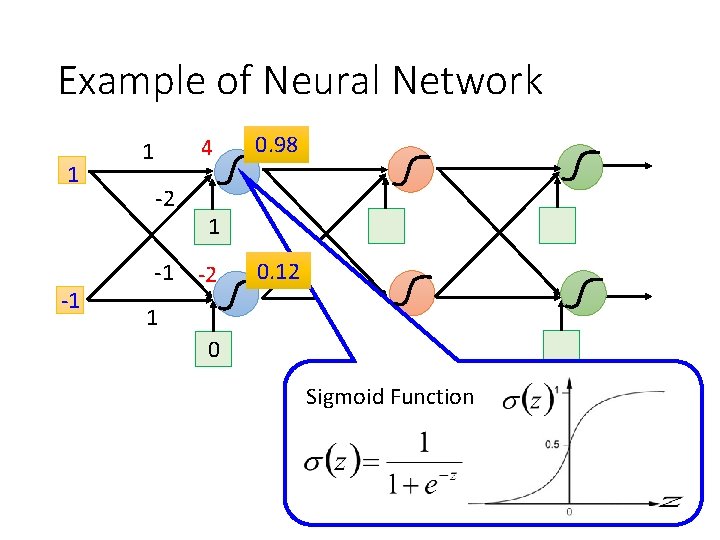
Example of Neural Network 1 -1 4 1 -2 -1 0. 98 1 -2 0. 12 1 0 Sigmoid Function

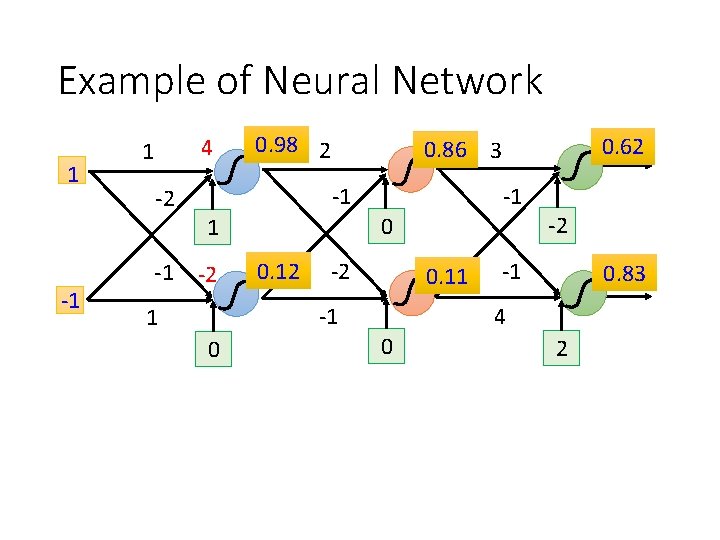
Example of Neural Network 1 -1 4 1 -2 -1 0. 98 2 -1 -1 0. 12 -2 0. 11 -1 1 0 -2 0 1 -2 0. 62 0. 86 3 -1 0. 83 4 0 2

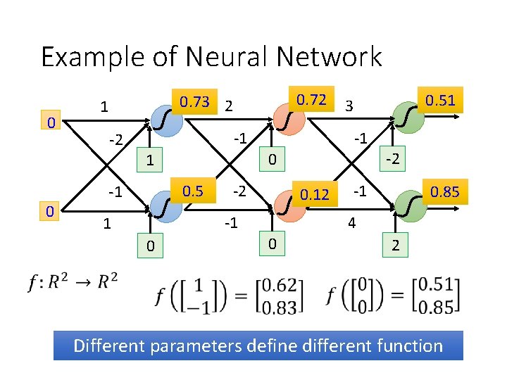
Example of Neural Network 0 0 0. 72 0. 73 2 1 -2 -1 -1 0. 5 -2 0. 12 -1 1 0 -2 0 1 -1 0. 51 3 -1 0. 85 4 0 2 Different parameters define different function

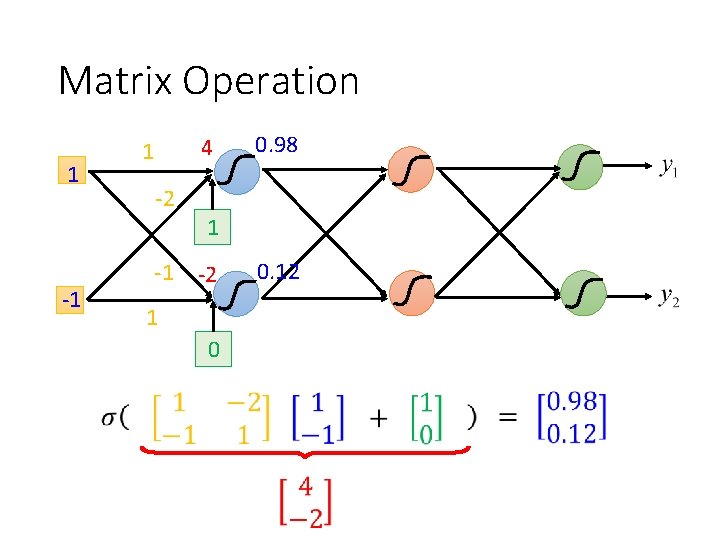
Matrix Operation 1 -1 4 1 -2 -1 0. 98 1 -2 1 0 0. 12

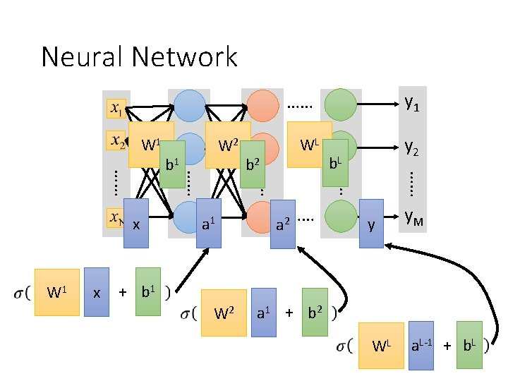
Neural Network W 1 WL …… y 2 + b 1 W 2 …… a 1 b. L …… x b 2 y 1 …… W 1 …… …… x b 1 W 2 …… y y. M a 1 + b 2 WL a. L-1 + b. L

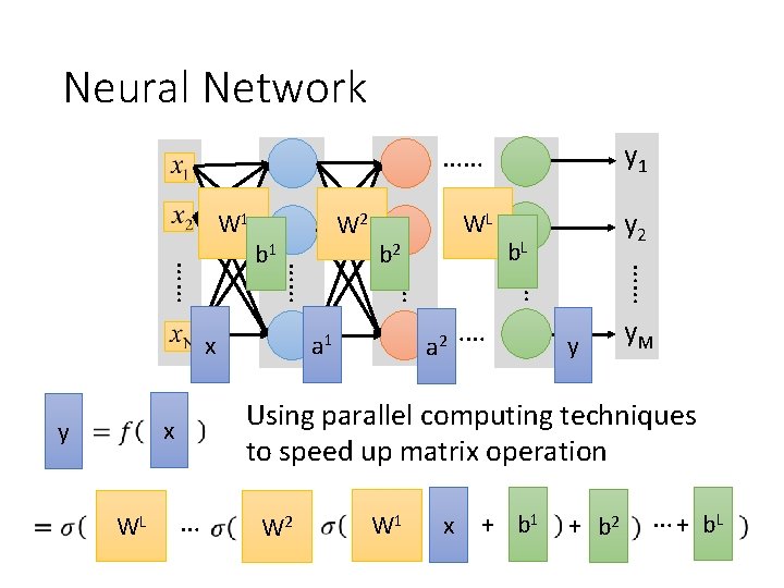
Neural Network W 1 b. L …… a 1 a 2 …… WL y 2 y y. M Using parallel computing techniques to speed up matrix operation x y WL …… …… x b 2 y 1 …… …… …… b 1 W 2 …… … W 2 W 1 x + b 1 + b 2 … + b. L

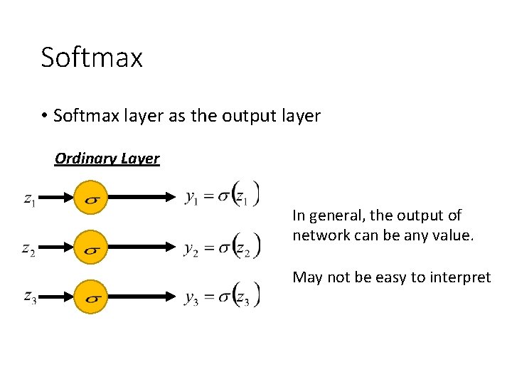
Softmax • Softmax layer as the output layer Ordinary Layer In general, the output of network can be any value. May not be easy to interpret

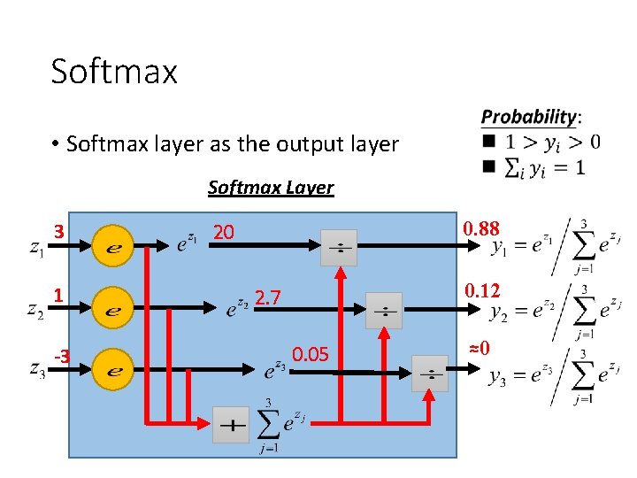
Softmax • Softmax layer as the output layer Softmax Layer 3 1 -3 0. 88 20 0. 12 2. 7 0. 05 ≈0

How to set network parameters …… 16 x 16 = 256 Ink → 1 No ink → 0 is 1 0. 7 y 2 is 2 …… …… Softmax …… y 1 0. 2 y 10 is 0 thethe neural Input: How to let y 1 has maximum value Input: network achieve this y 2 has the maximum value

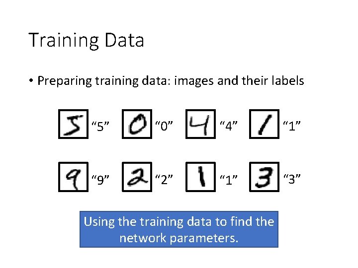
Training Data • Preparing training data: images and their labels “ 5” “ 0” “ 4” “ 1” “ 9” “ 2” “ 1” “ 3” Using the training data to find the network parameters.

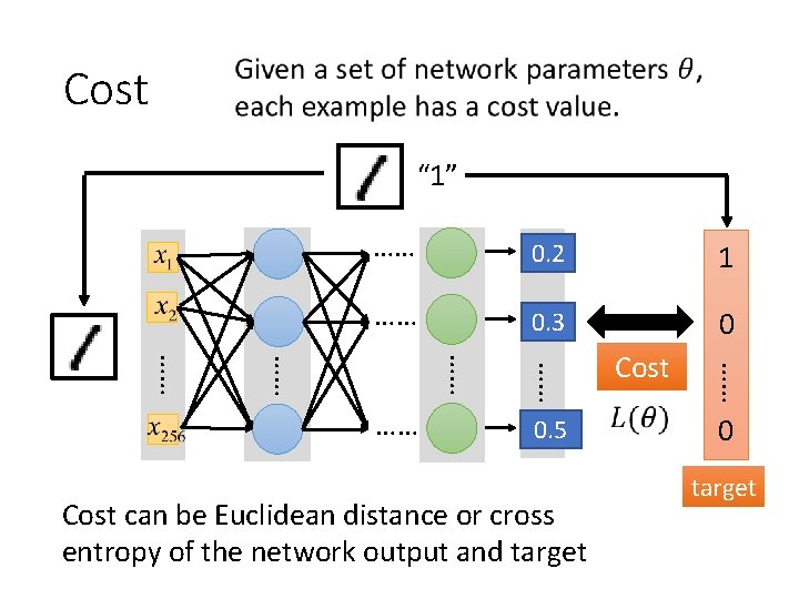
Cost “ 1” …… y 0. 2 1 1 …… 0. 3 y 2 0 y 0. 5 10 Cost can be Euclidean distance or cross entropy of the network output and target …… …… …… Cost 0 target

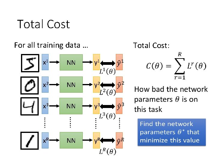
Total Cost For all training data … Total Cost: NN y 1 x 2 NN y 2 x 3 NN y 3 …… …… …… x. R NN y. R …… x 1

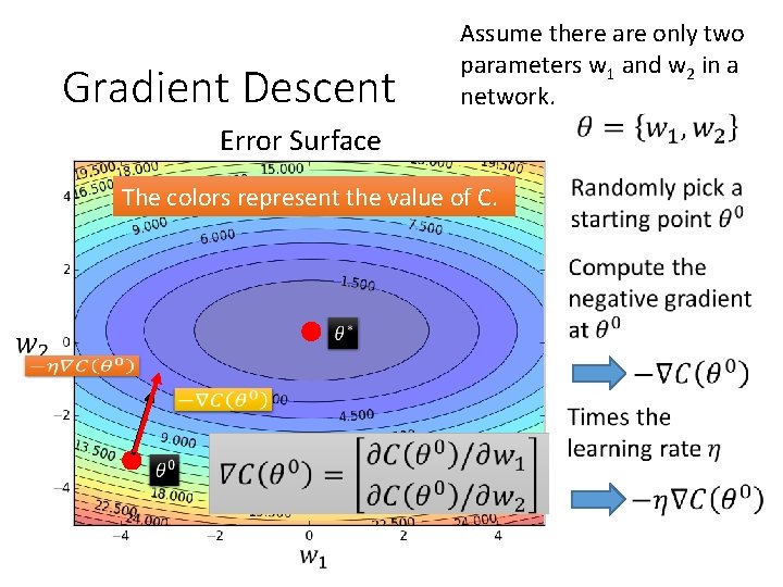
Gradient Descent Assume there are only two parameters w 1 and w 2 in a network. Error Surface The colors represent the value of C.

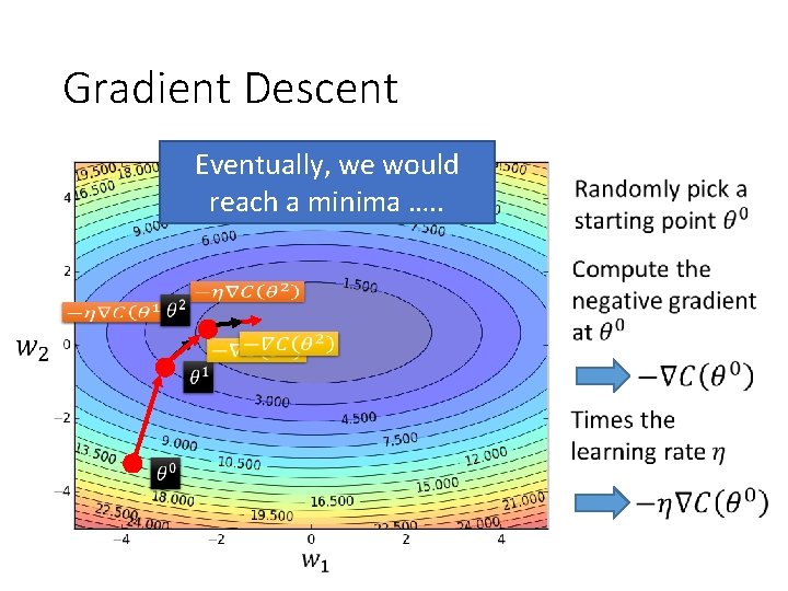
Gradient Descent Eventually, we would reach a minima …. .

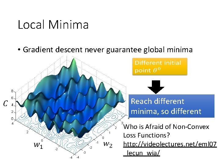
Local Minima • Gradient descent never guarantee global minima Reach different minima, so different results Who is Afraid of Non-Convex Loss Functions? http: //videolectures. net/eml 07 _lecun_wia/

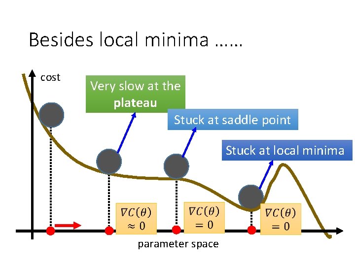
Besides local minima …… cost Very slow at the plateau Stuck at saddle point Stuck at local minima parameter space

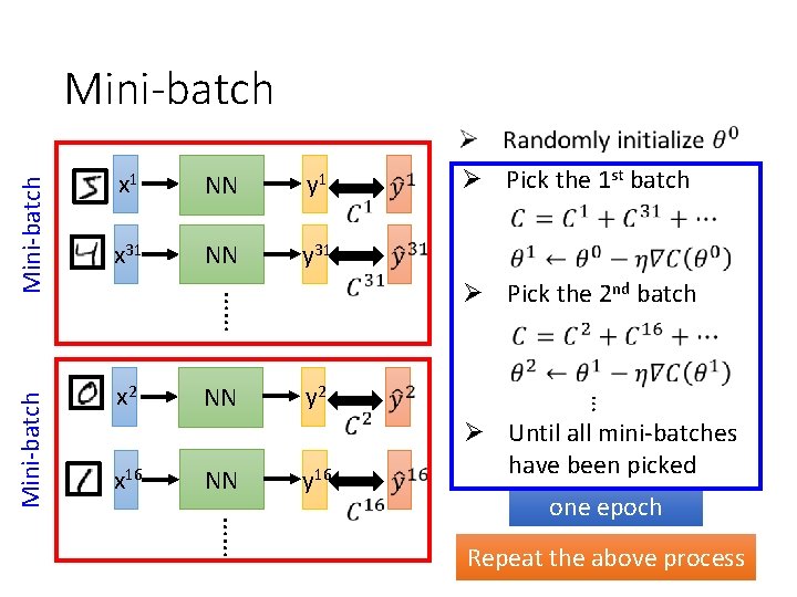
NN y 1 x 31 NN y 31 x 2 x 16 NN NN Ø Pick the 1 st batch Ø Pick the 2 nd batch y 2 y 16 … Mini-batch x 1 …… Mini-batch Ø Until all mini-batches have been picked …… one epoch Repeat the above process

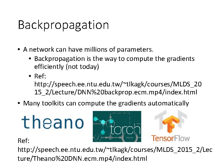
Backpropagation • A network can have millions of parameters. • Backpropagation is the way to compute the gradients efficiently (not today) • Ref: http: //speech. ee. ntu. edu. tw/~tlkagk/courses/MLDS_20 15_2/Lecture/DNN%20 backprop. ecm. mp 4/index. html • Many toolkits can compute the gradients automatically Ref: http: //speech. ee. ntu. edu. tw/~tlkagk/courses/MLDS_2015_2/Lec ture/Theano%20 DNN. ecm. mp 4/index. html

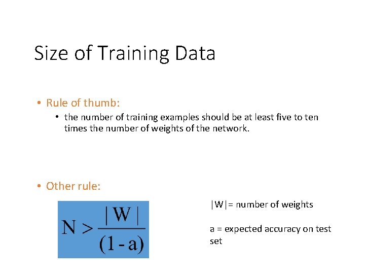
Size of Training Data • Rule of thumb: • the number of training examples should be at least five to ten times the number of weights of the network. • Other rule: |W|= number of weights a = expected accuracy on test set

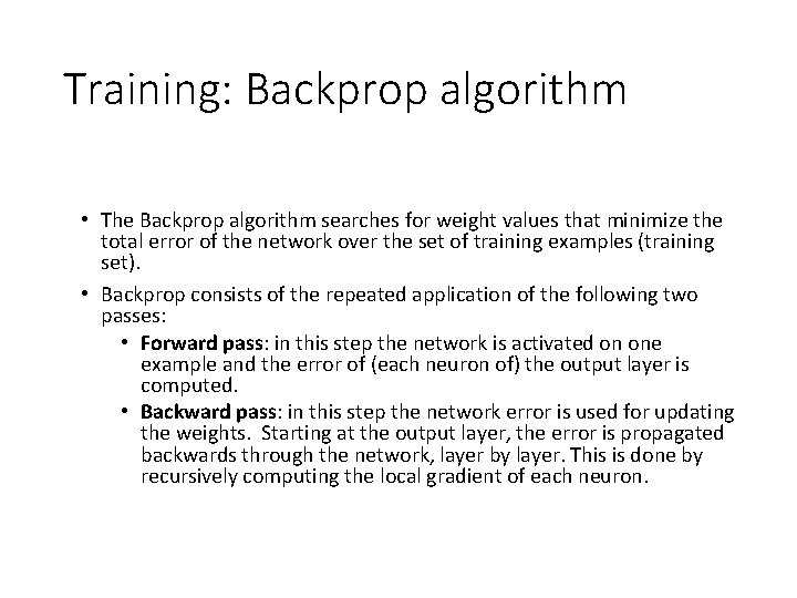
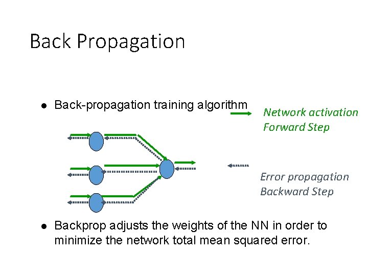
Training: Backprop algorithm • The Backprop algorithm searches for weight values that minimize the total error of the network over the set of training examples (training set). • Backprop consists of the repeated application of the following two passes: • Forward pass: in this step the network is activated on one example and the error of (each neuron of) the output layer is computed. • Backward pass: in this step the network error is used for updating the weights. Starting at the output layer, the error is propagated backwards through the network, layer by layer. This is done by recursively computing the local gradient of each neuron.

Back Propagation l Back-propagation training algorithm Network activation Forward Step Error propagation Backward Step l Backprop adjusts the weights of the NN in order to minimize the network total mean squared error.

Part II: Why Deep?

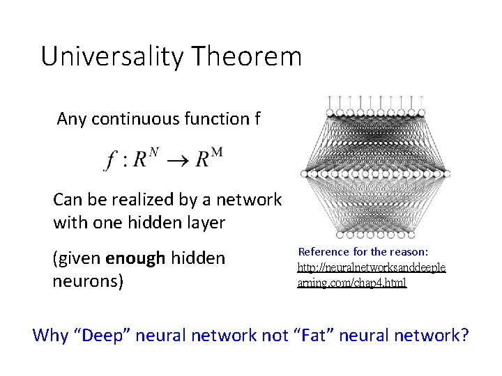
Universality Theorem Any continuous function f Can be realized by a network with one hidden layer (given enough hidden neurons) Reference for the reason: http: //neuralnetworksanddeeple arning. com/chap 4. html Why “Deep” neural network not “Fat” neural network?

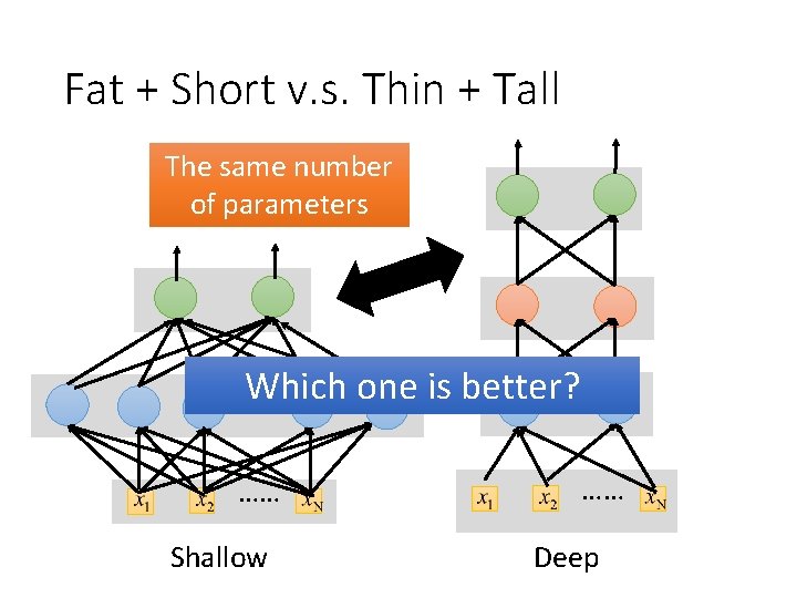
Fat + Short v. s. Thin + Tall The same number of parameters Which one is better? …… …… Shallow …… Deep

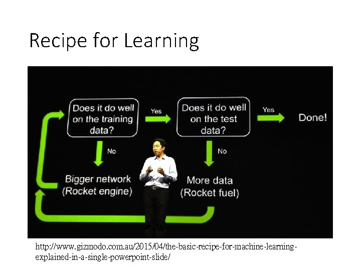
Recipe for Learning http: //www. gizmodo. com. au/2015/04/the-basic-recipe-for-machine-learningexplained-in-a-single-powerpoint-slide/

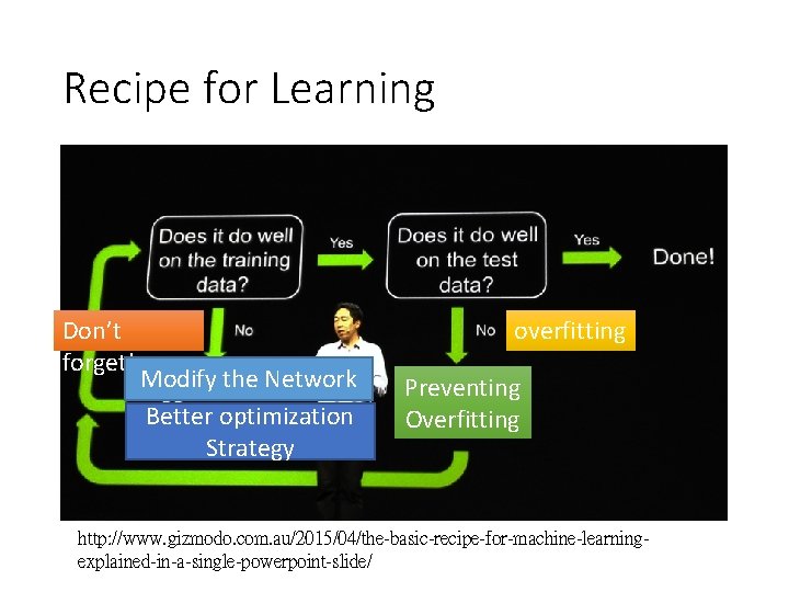
Recipe for Learning Don’t forget! overfitting Modify the Network Better optimization Strategy Preventing Overfitting http: //www. gizmodo. com. au/2015/04/the-basic-recipe-for-machine-learningexplained-in-a-single-powerpoint-slide/

Neural networks re-visited

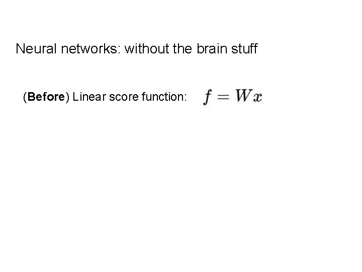
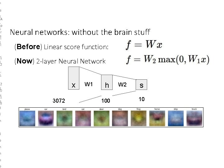
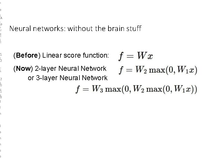
Neural networks: without the brain stuff (Before) Linear score function:

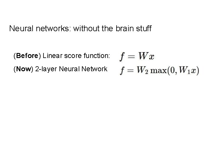
Neural networks: without the brain stuff (Before) Linear score function: (Now) 2 -layer Neural Network

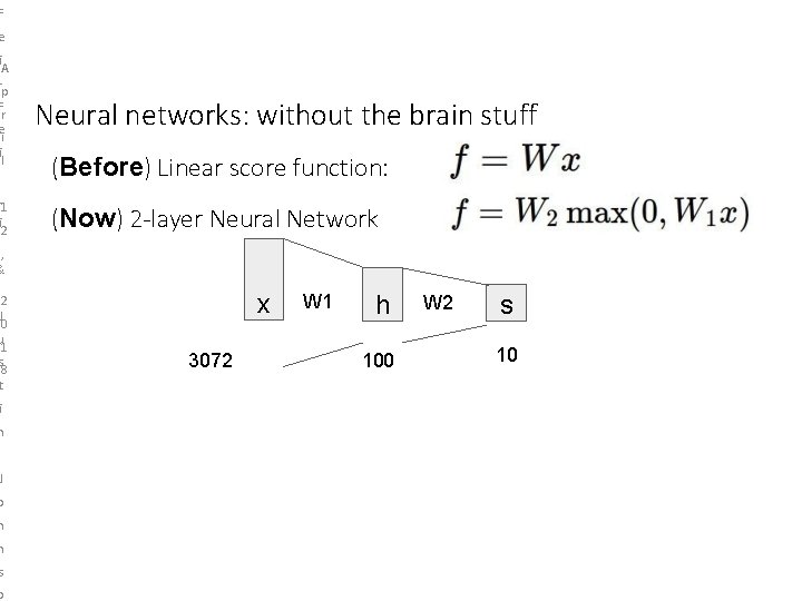
F e i LA ep F r e ti i ul r L e 1 i 2 Neural networks: without the brain stuff (Before) Linear score function: (Now) 2 -layer Neural Network , & -2 J 0 u 1 s 8 t i n J o h n s o x 3072 W 1 h 100 W 2 s 10

F e i LA ep F r e ti i ul r L e 1 i 2 Neural networks: without the brain stuff (Before) Linear score function: (Now) 2 -layer Neural Network , & -2 J 0 u 1 s 8 t i n J o h n s o x 3072 W 1 h 100 W 2 s 10

F e i LA ep F r e ti i ul r L e 1 i 2 , & -2 J 0 u 1 s 8 t i n J o h n s o Neural networks: without the brain stuff (Before) Linear score function: (Now) 2 -layer Neural Network or 3 -layer Neural Network

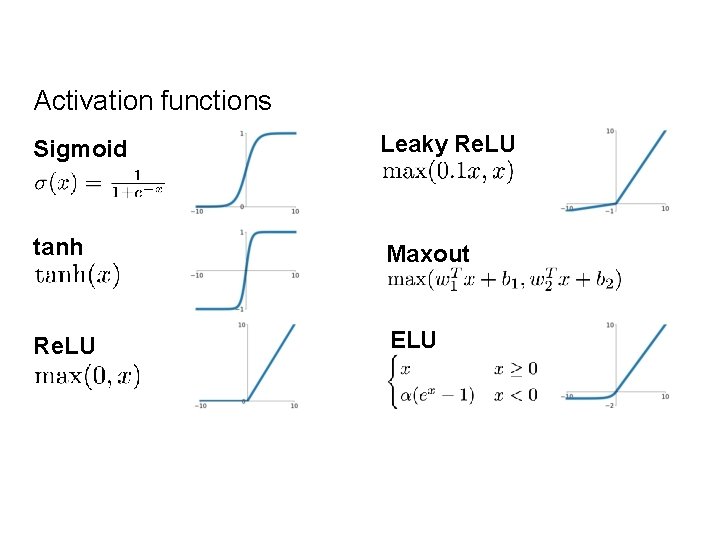
Activation functions Sigmoid Leaky Re. LU tanh Maxout Re. LU ELU

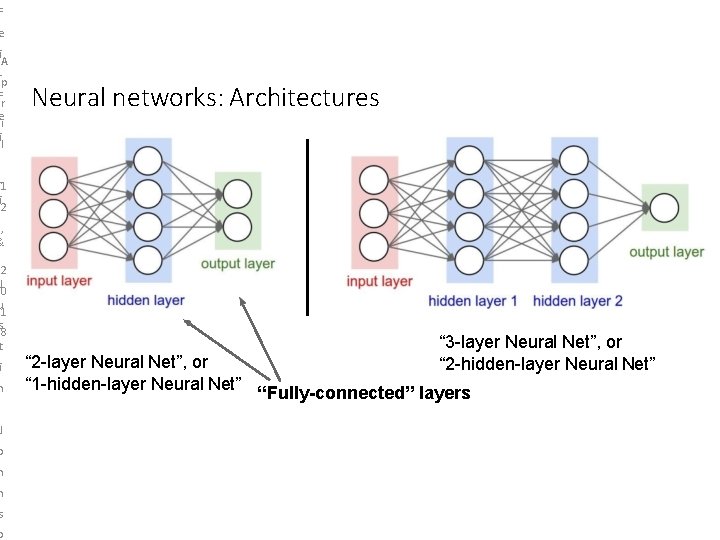
F e i LA ep F r e ti i ul Neural networks: Architectures r L e 1 i 2 , & -2 J 0 u 1 s 8 t i n J o h n s o “ 3 -layer Neural Net”, or “ 2 -hidden-layer Neural Net” “ 2 -layer Neural Net”, or “ 1 -hidden-layer Neural Net” “Fully-connected” layers

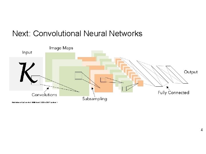
Next: Convolutional Neural Networks Illustration of Le. Cun et al. 1998 from CS 231 n 2017 Lecture 1 Lecture 5 - 7 3 April 17, 20184

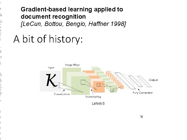
F e i. A p F r e i i l L Gradient-based learning applied to document recognition [Le. Cun, Bottou, Bengio, Haffner 1998] A bit of history: i 1 7 &, J 2 u 0 s 1 t 8 i n Le. Net-5 J o h n s o Lecture 5 - 1144

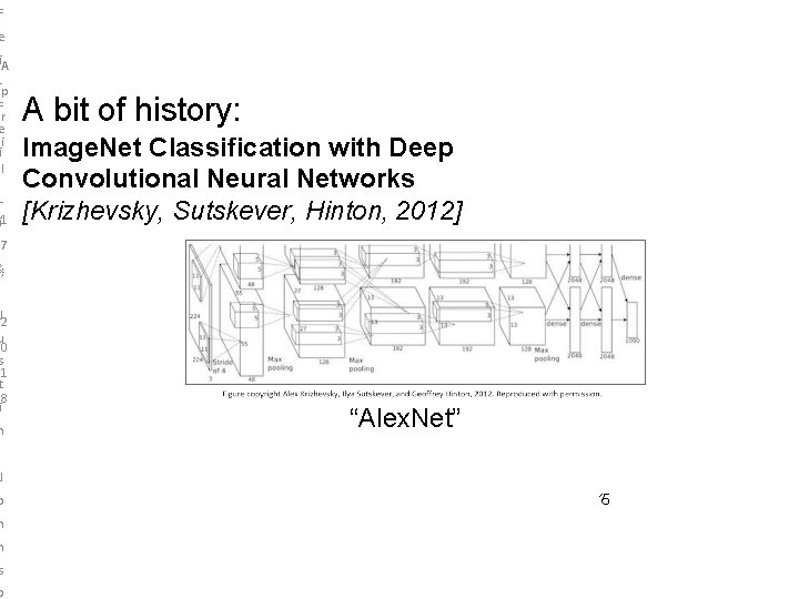
F e i. A p F r e i i l L i 1 A bit of history: Image. Net Classification with Deep Convolutional Neural Networks [Krizhevsky, Sutskever, Hinton, 2012] 7 &, J 2 u 0 s 1 t 8 i n “Alex. Net” J o h n s o Lecture 5 - 1155

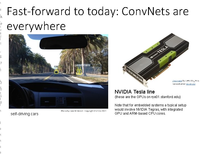
F e Li. A e-p F cer tii ul r. L ei 1 Fast-forward to today: Conv. Nets are everywhere 7 &, J 2 u 0 s 1 t 8 i n NVIDIA Tesla line (these are the GPUs on rye 01. stanford. edu) self-driving cars Note that for embedded systems a typical setup would involve NVIDIA Tegras, with integrated GPU and ARM-based CPU cores. J o h n s o Fei-Fei Li & Justin Johnson & Serena Yeung Lecture 5 - April 17, 2018

F e Li. A e-p F cer tii ul r. L ei 1 7 &, J 2 u 0 s 1 t 8 i Convolutional Neural Networks (First without the brain stuff) n J o h n s o Fei-Fei Li & Justin Johnson & Serena Yeung Lecture 5 - April 17, 2018

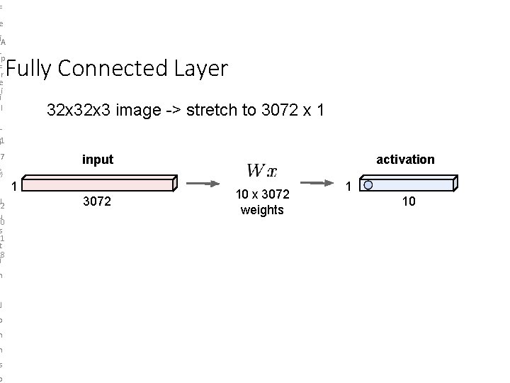
F e Li. A e-p F cer tii ul r. L ei 1 Fully Connected Layer 32 x 3 image -> stretch to 3072 x 1 7 input activation &, J 2 u 0 s 1 t 8 i 1 3072 10 x 3072 weights 1 10 n J o h n s o Fei-Fei Li & Justin Johnson & Serena Yeung Lecture 5 - April 17, 2018

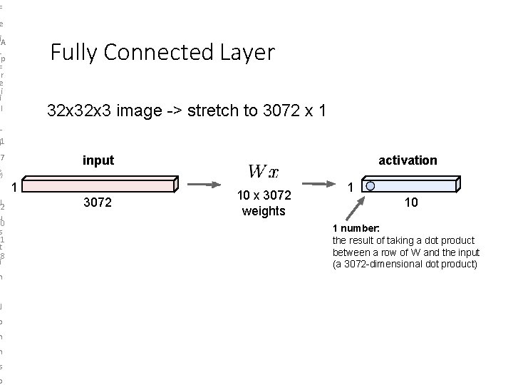
F e Li. A e-p F cer tii ul r. L ei 1 Fully Connected Layer 32 x 3 image -> stretch to 3072 x 1 7 input activation &, J 2 u 0 s 1 t 8 i 1 3072 10 x 3072 weights 1 10 1 number: the result of taking a dot product between a row of W and the input (a 3072 -dimensional dot product) n J o h n s o Fei-Fei Li & Justin Johnson & Serena Yeung Lecture 5 - April 17, 2018

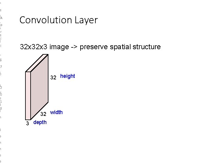
F e Li. A e-p F cer tii ul r. L ei 1 Convolution Layer 32 x 3 image -> preserve spatial structure 7 &, J 2 u 0 s 1 t 8 i n 32 height 32 width 3 depth J o h n s o Fei-Fei Li & Justin Johnson & Serena Yeung Lecture 5 - April 17, 2018

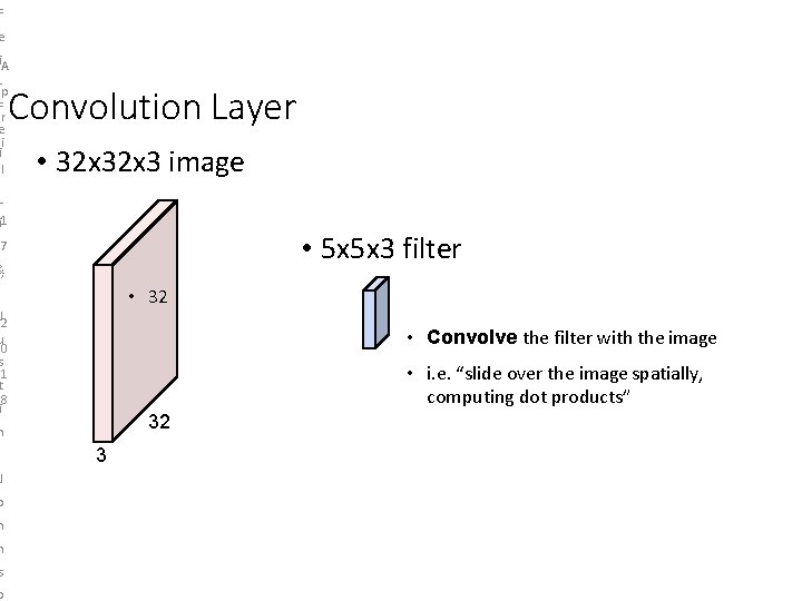
F e Li. A e-p F cer tii ul r. L ei 1 Convolution Layer • 32 x 3 image • 5 x 5 x 3 filter 7 &, • 32 J 2 u 0 s 1 t 8 i • Convolve the filter with the image • i. e. “slide over the image spatially, computing dot products” 32 n 3 J o h n s o Fei-Fei Li & Justin Johnson & Serena Yeung Lecture 5 - April 17, 2018

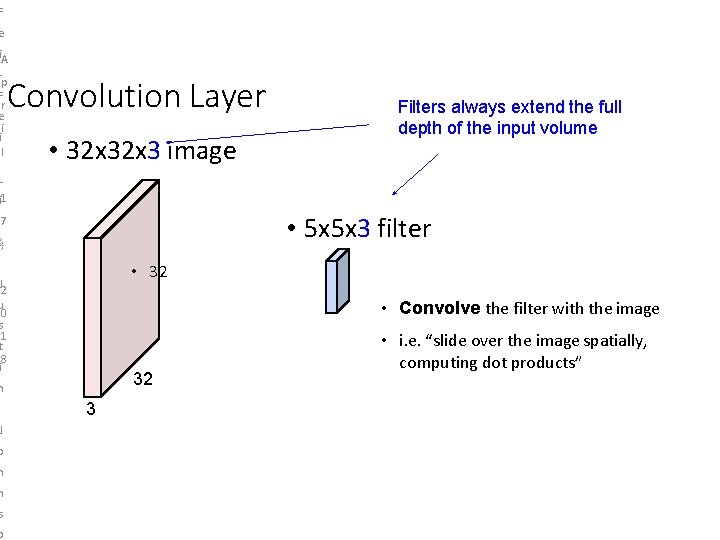
F e Li. A e-p F cer tii ul r. L ei 1 Convolution Layer Filters always extend the full depth of the input volume • 32 x 3 image • 5 x 5 x 3 filter 7 &, • 32 J 2 u 0 s 1 t 8 i • Convolve the filter with the image 32 n • i. e. “slide over the image spatially, computing dot products” 3 J o h n s o Fei-Fei Li & Justin Johnson & Serena Yeung Lecture 5 - April 17, 2018

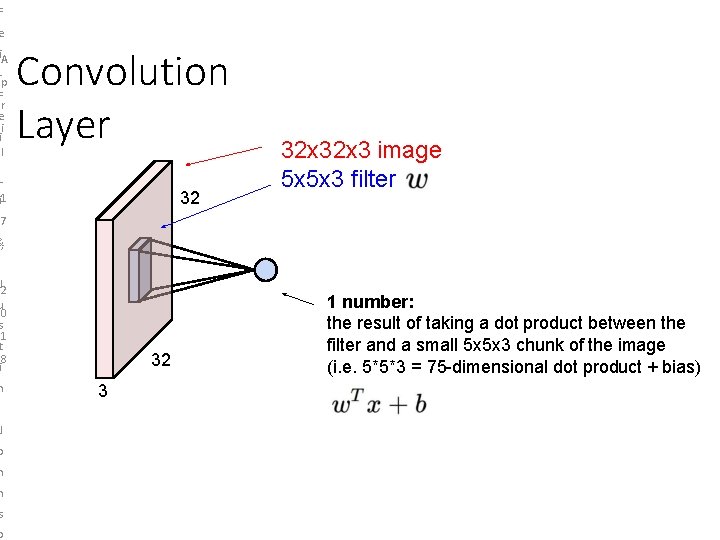
F e Li. A e-p F cer tii ul r. L ei 1 Convolution Layer 32 32 x 3 image 5 x 5 x 3 filter 7 &, J 2 u 0 s 1 t 8 i n 32 1 number: the result of taking a dot product between the filter and a small 5 x 5 x 3 chunk of the image (i. e. 5*5*3 = 75 -dimensional dot product + bias) 3 J o h n s o Fei-Fei Li & Justin Johnson & Serena Yeung Lecture 5 - April 17, 2018

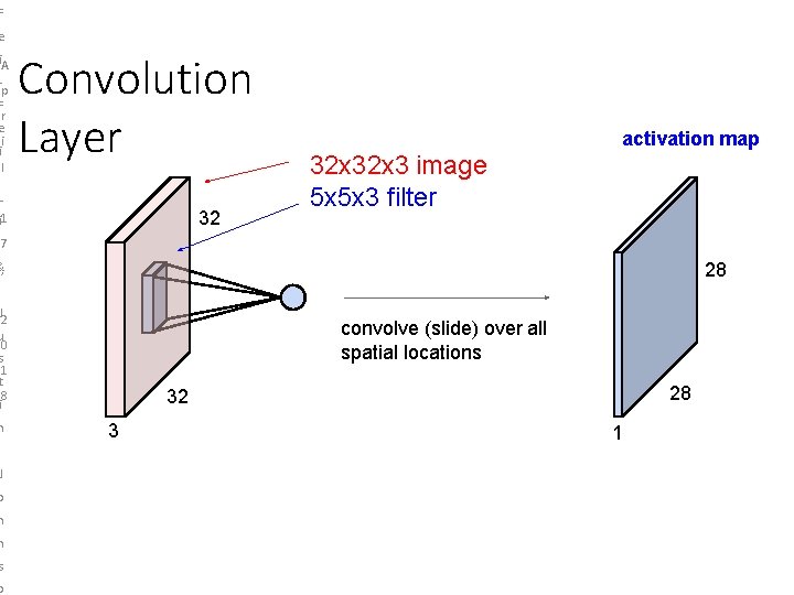
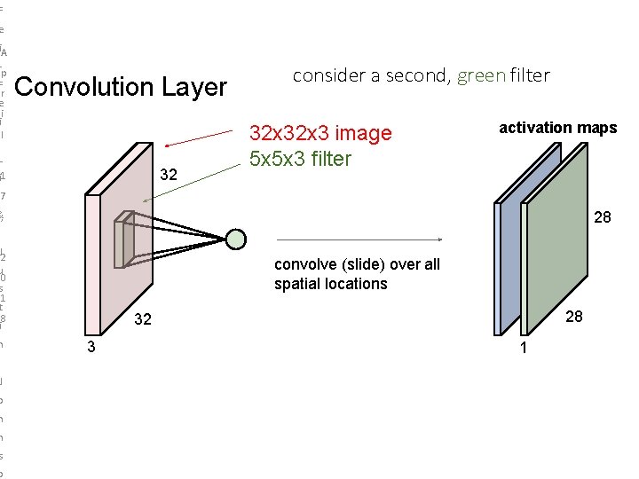
F e Li. A e-p F cer tii ul r. L ei 1 Convolution Layer 32 activation map 32 x 3 image 5 x 5 x 3 filter 7 &, 28 J 2 u 0 s 1 t 8 i n convolve (slide) over all spatial locations 28 32 3 1 J o h n s o Fei-Fei Li & Justin Johnson & Serena Yeung Lecture 5 - April 17, 2018

F e i. A p F r e i i l Convolution Layer L 32 i 1 consider a second, green filter 32 x 3 image 5 x 5 x 3 filter activation maps 7 &, 28 J 2 u 0 s 1 t 8 i n convolve (slide) over all spatial locations 28 32 3 1 J o h n s o Fei-Fei Li & Justin Johnson & Serena Yeung Lecture 5 - 33 April 17, 2018

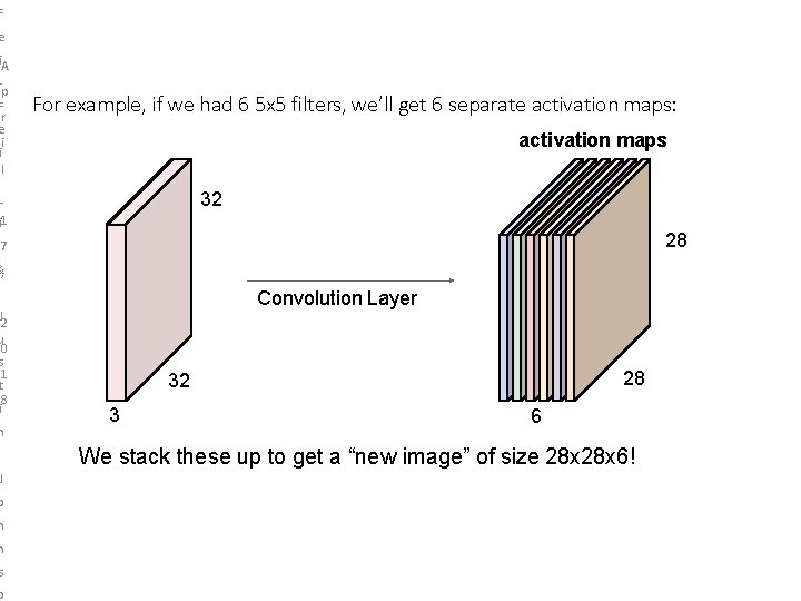
F e Li. A e-p F cer tii ul r. L ei 1 For example, if we had 6 5 x 5 filters, we’ll get 6 separate activation maps: activation maps 32 28 7 &, J 2 u 0 s 1 t 8 i n Convolution Layer 28 32 3 6 We stack these up to get a “new image” of size 28 x 6! J o h n s o Fei-Fei Li & Justin Johnson & Serena Yeung Lecture 5 - April 17, 2018

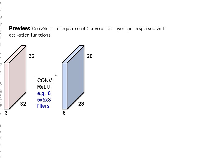
F e Li. A e-p F cer tii ul r. L ei 1 Preview: Conv. Net is a sequence of Convolution Layers, interspersed with activation functions 32 28 7 &, J 2 u 0 s 1 t 8 i n 32 3 CONV, Re. LU e. g. 6 5 x 5 x 3 filters 28 6 J o h n s o Fei-Fei Li & Justin Johnson & Serena Yeung Lecture 5 - April 17, 2018

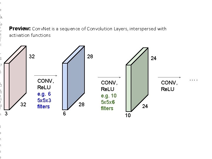
F e Li. A e-p F cer tii ul r. L ei 1 Preview: Conv. Net is a sequence of Convolution Layers, interspersed with activation functions 32 28 24 7 &, J 2 u 0 s 1 t 8 i n 32 3 CONV, Re. LU e. g. 6 5 x 5 x 3 filters 28 6 CONV, Re. LU e. g. 10 5 x 5 x 6 filters CONV, Re. LU …. 24 10 J o h n s o Fei-Fei Li & Justin Johnson & Serena Yeung Lecture 5 - April 17, 2018

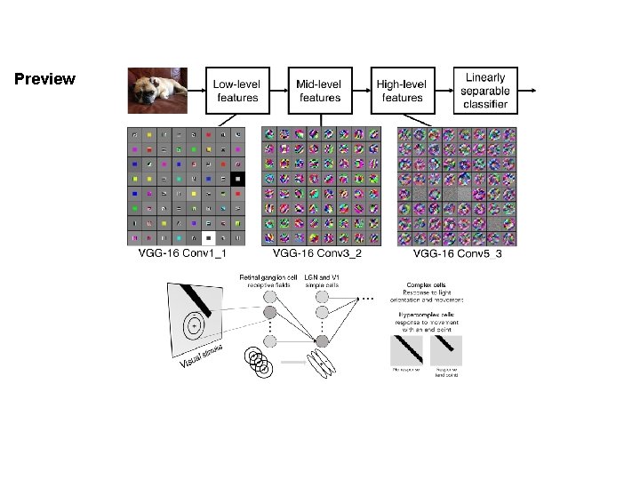
Preview Fei-Fei Li & Justin Johnson & Serena Yeung [Zeiler and Fergus 2013] Lecture 5 - April 17, 2018

Preview Fei-Fei Li & Justin Johnson & Serena Yeung Lecture 5 - April 17, 2018

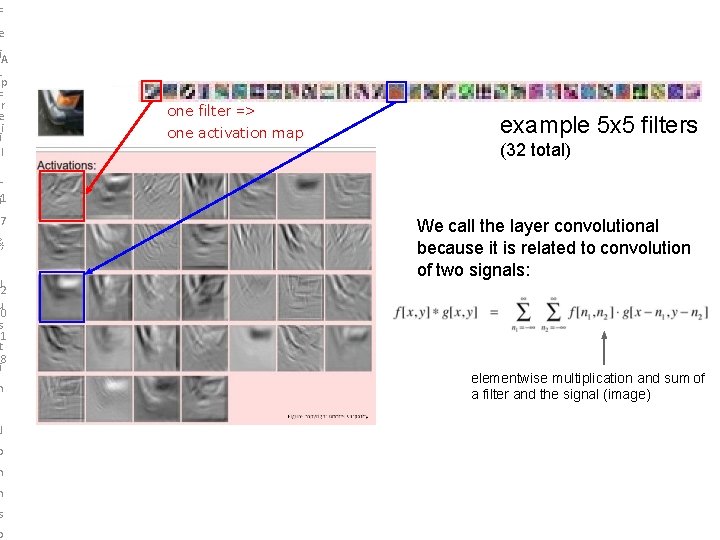
F e Li. A e-p F cer tii ul r. L ei 1 one filter => one activation map 7 example 5 x 5 filters (32 total) We call the layer convolutional because it is related to convolution of two signals: &, J 2 u 0 s 1 t 8 i elementwise multiplication and sum of a filter and the signal (image) n J o h n s o Fei-Fei Li & Justin Johnson & Serena Yeung Lecture 5 - April 17, 2018

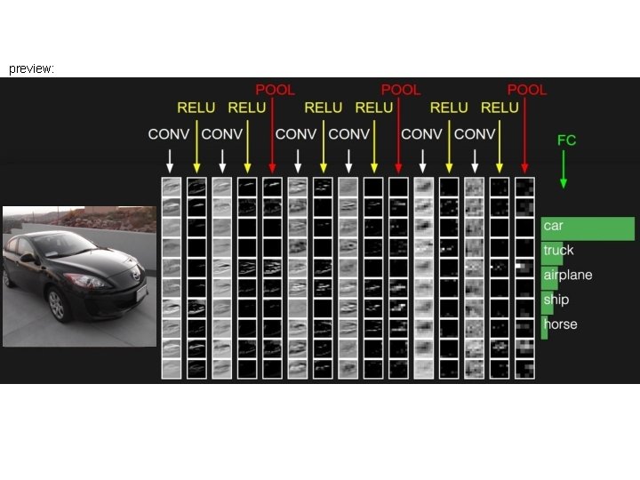
preview: Fei-Fei Li & Justin Johnson & Serena Yeung Lecture 5 - April 17, 2018

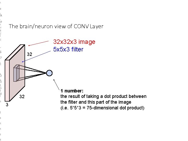
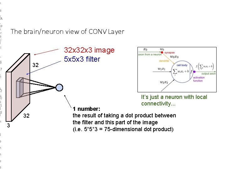
F e Li. A e-p F cer tii ul r. L ei 1 The brain/neuron view of CONV Layer 32 7 32 x 3 image 5 x 5 x 3 filter &, J 2 u 0 s 1 t 8 i n 32 3 1 number: the result of taking a dot product between the filter and this part of the image (i. e. 5*5*3 = 75 -dimensional dot product) J o h n s o Fei-Fei Li & Justin Johnson & Serena Yeung Lecture 5 - April 17, 2018

F e Li. A e-p F cer tii ul r. L ei 1 The brain/neuron view of CONV Layer 32 7 32 x 3 image 5 x 5 x 3 filter &, J 2 u 0 s 1 t 8 i n It’s just a neuron with local connectivity. . . 32 3 1 number: the result of taking a dot product between the filter and this part of the image (i. e. 5*5*3 = 75 -dimensional dot product) J o h n s o Fei-Fei Li & Justin Johnson & Serena Yeung Lecture 5 - April 17, 2018

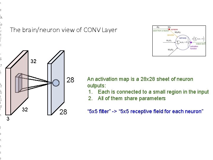
F e Li. A e-p F cer tii ul r. L ei 1 The brain/neuron view of CONV Layer 32 7 &, 28 J 2 u 0 s 1 t 8 i n 32 3 28 An activation map is a 28 x 28 sheet of neuron outputs: 1. Each is connected to a small region in the input 2. All of them share parameters “ 5 x 5 filter” -> “ 5 x 5 receptive field for each neuron” J o h n s o Fei-Fei Li & Justin Johnson & Serena Yeung Lecture 5 - April 17, 2018

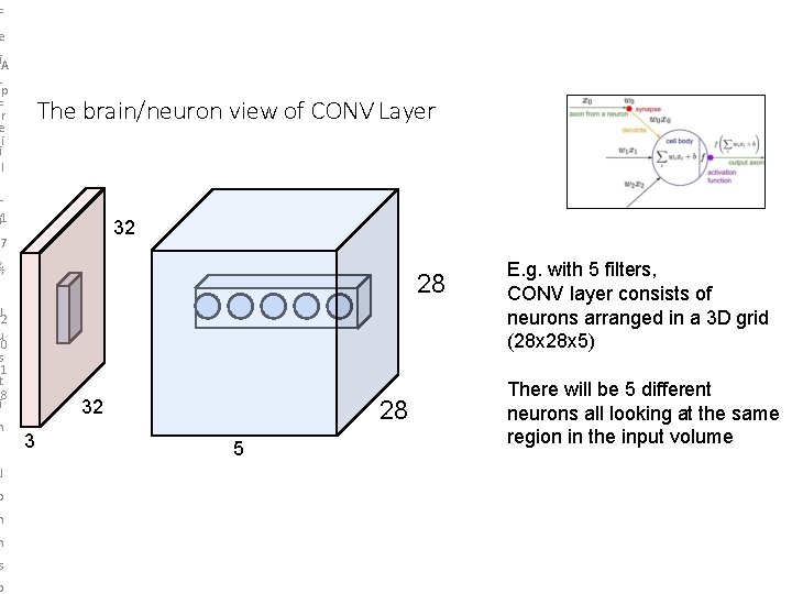
F e Li. A e-p F cer tii ul r. L ei 1 The brain/neuron view of CONV Layer 32 7 &, 28 J 2 u 0 s 1 t 8 i n 32 3 28 5 E. g. with 5 filters, CONV layer consists of neurons arranged in a 3 D grid (28 x 5) There will be 5 different neurons all looking at the same region in the input volume J o h n s o Fei-Fei Li & Justin Johnson & Serena Yeung Lecture 5 - April 17, 2018

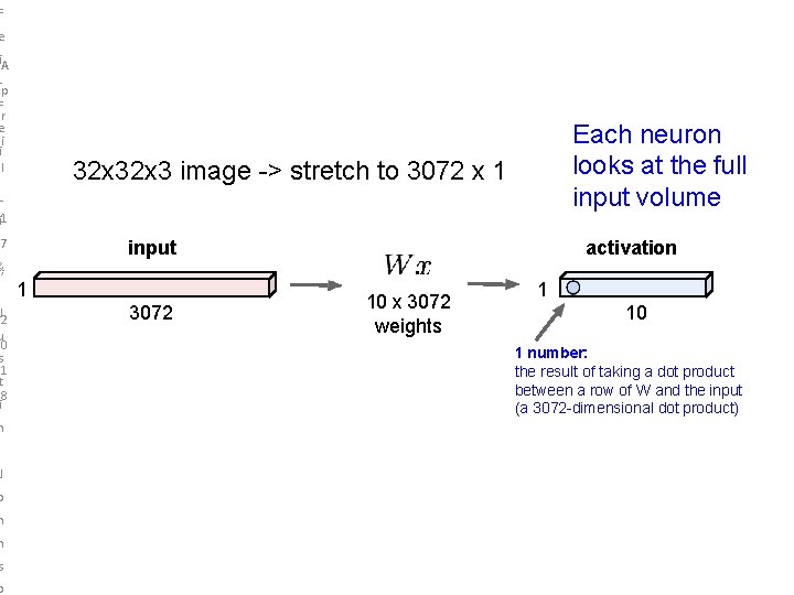
F e Li. A e-p F cer tii ul r. L ei 1 Each neuron looks at the full input volume 32 x 3 image -> stretch to 3072 x 1 7 input activation &, J 2 u 0 s 1 t 8 i 1 3072 10 x 3072 weights 1 10 1 number: the result of taking a dot product between a row of W and the input (a 3072 -dimensional dot product) n J o h n s o Fei-Fei Li & Justin Johnson & Serena Yeung Lecture 5 - April 17, 2018

two more layers to go: POOL/FC Fei-Fei Li & Justin Johnson & Serena Yeung Lecture 5 - April 17, 2018

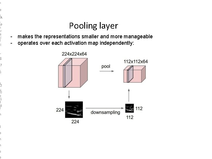
F e Li. A e-p F cer tii ul r. L ei 1 Pooling layer - makes the representations smaller and more manageable - operates over each activation map independently: 7 &, J 2 u 0 s 1 t 8 i n J o h n s o Fei-Fei Li & Justin Johnson & Serena Yeung Lecture 5 - April 17, 2018

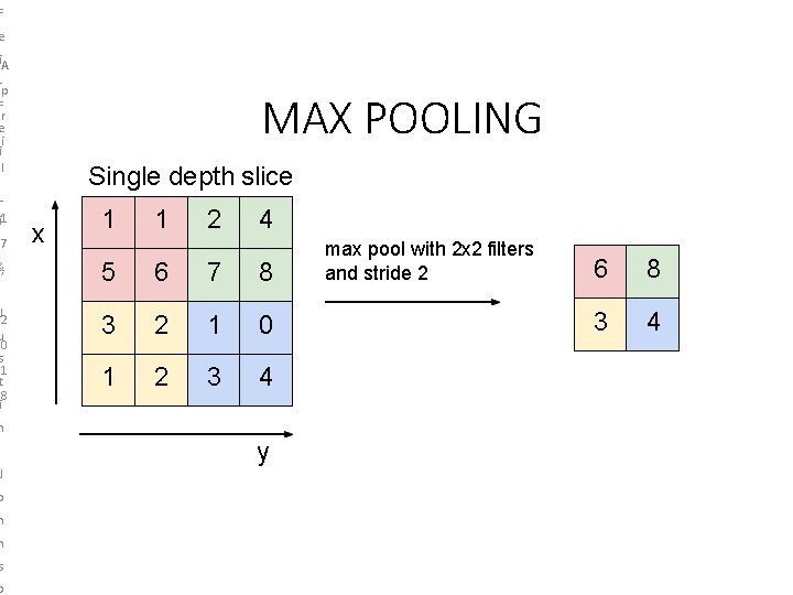
F e Li A e-p c. Fr tei uil r L ei 1 7 MAX POOLING Single depth slice x 1 1 2 4 &, 5 6 7 8 J 2 u 0 s 1 t 8 i 3 2 1 0 1 2 3 4 max pool with 2 x 2 filters and stride 2 6 8 3 4 n J o h n s o y Fei-Fei Li & Justin Johnson & Serena Yeung Lecture 5 - April 17, 2018

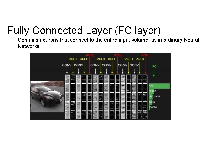
Fully Connected Layer (FC layer) - Contains neurons that connect to the entire input volume, as in ordinary Neural Networks Fei-Fei Li & Justin Johnson & Serena Yeung Lecture 5 - April 17, 2018

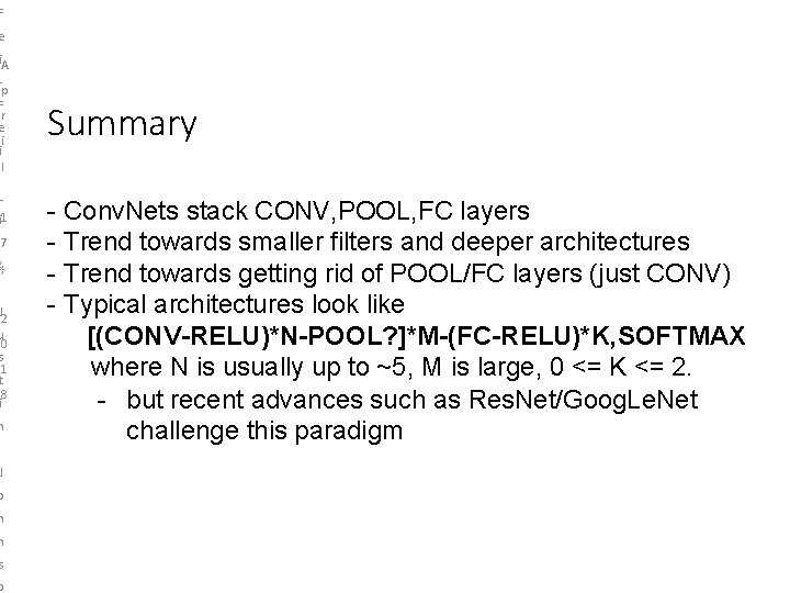
F e Li A e-p c. Fr tei uil r L ei 1 7 &, J 2 u 0 s 1 t 8 i n Summary - Conv. Nets stack CONV, POOL, FC layers - Trend towards smaller filters and deeper architectures - Trend towards getting rid of POOL/FC layers (just CONV) - Typical architectures look like [(CONV-RELU)*N-POOL? ]*M-(FC-RELU)*K, SOFTMAX where N is usually up to ~5, M is large, 0 <= K <= 2. - but recent advances such as Res. Net/Goog. Le. Net challenge this paradigm J o h n s o Fei-Fei Li & Justin Johnson & Serena Yeung Lecture 5 - April 17, 2018