ECE 8443 Pattern Recognition LECTURE 12 HIDDEN MARKOV

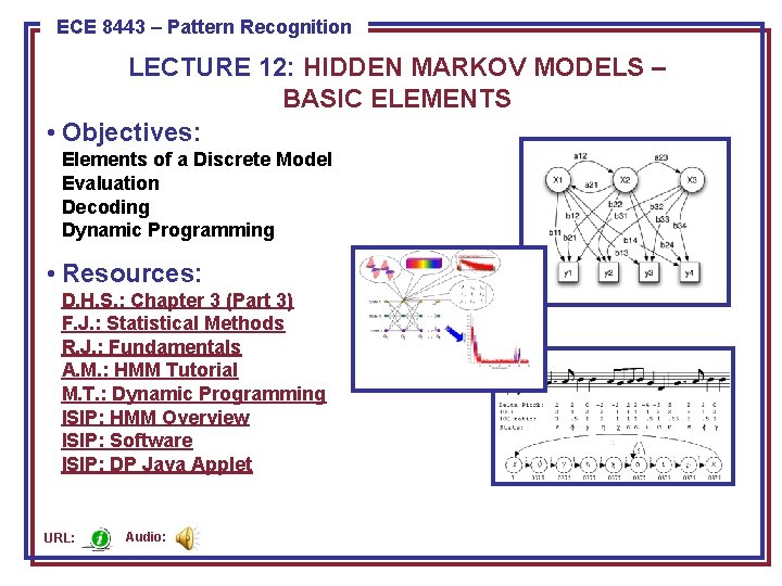
ECE 8443 – Pattern Recognition LECTURE 12: HIDDEN MARKOV MODELS – BASIC ELEMENTS • Objectives: Elements of a Discrete Model Evaluation Decoding Dynamic Programming • Resources: D. H. S. : Chapter 3 (Part 3) F. J. : Statistical Methods R. J. : Fundamentals A. M. : HMM Tutorial M. T. : Dynamic Programming ISIP: HMM Overview ISIP: Software ISIP: DP Java Applet URL: Audio:

Motivation • Thus far we have dealt with parameter estimation for the static pattern classification problem: estimating the parameters of class-conditional densities needed to make a single decision. • Many problems have an inherent temporal dimension – the vectors of interest come from a time series that unfolds as a function of time. Modeling temporal relationships between these vectors is an important part of the problem. • Markov models are a popular way to model such signals. There are many generalizations of these approaches, including Markov Random Fields and Bayesian Networks. § First-order Markov processes are very effective because they are sufficiently powerful and computationally efficient. § Higher-order Markov processes can be represented using first-order processes • Markov models are very attractive because of their ability to automatically learn underlying structure. Often this structure has relevance to the pattern recognition problem (e. g. , the states represents physical attributes of the system that generated the data). ECE 8443: Lecture 12, Slide 1

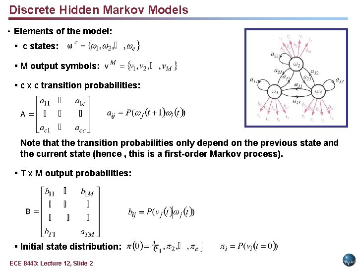
Discrete Hidden Markov Models • Elements of the model: § c states: § M output symbols: § c x c transition probabilities: Note that the transition probabilities only depend on the previous state and the current state (hence , this is a first-order Markov process). § T x M output probabilities: § Initial state distribution: ECE 8443: Lecture 12, Slide 2

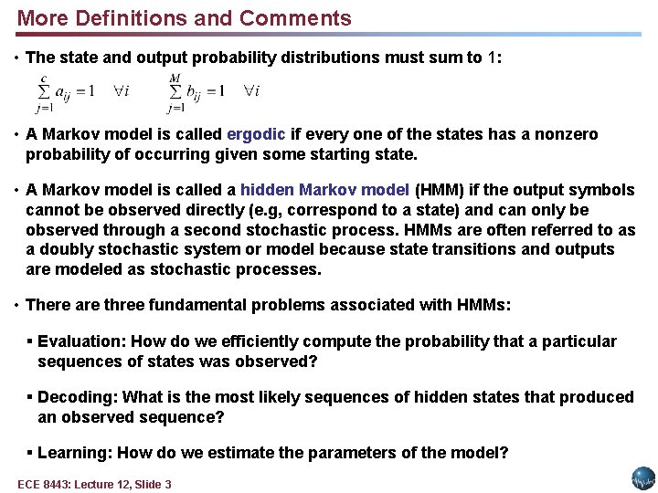
More Definitions and Comments • The state and output probability distributions must sum to 1: • A Markov model is called ergodic if every one of the states has a nonzero probability of occurring given some starting state. • A Markov model is called a hidden Markov model (HMM) if the output symbols cannot be observed directly (e. g, correspond to a state) and can only be observed through a second stochastic process. HMMs are often referred to as a doubly stochastic system or model because state transitions and outputs are modeled as stochastic processes. • There are three fundamental problems associated with HMMs: § Evaluation: How do we efficiently compute the probability that a particular sequences of states was observed? § Decoding: What is the most likely sequences of hidden states that produced an observed sequence? § Learning: How do we estimate the parameters of the model? ECE 8443: Lecture 12, Slide 3

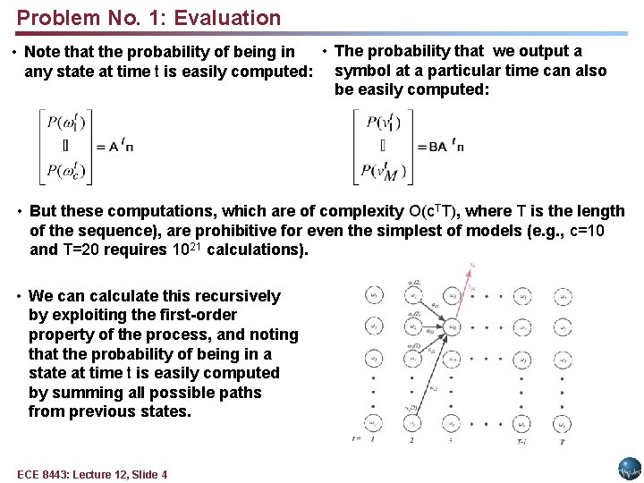
Problem No. 1: Evaluation • The probability that we output a • Note that the probability of being in any state at time t is easily computed: symbol at a particular time can also be easily computed: • But these computations, which are of complexity O(c. TT), where T is the length of the sequence), are prohibitive for even the simplest of models (e. g. , c=10 and T=20 requires 1021 calculations). • We can calculate this recursively by exploiting the first-order property of the process, and noting that the probability of being in a state at time t is easily computed by summing all possible paths from previous states. ECE 8443: Lecture 12, Slide 4

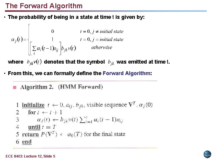
The Forward Algorithm • The probability of being in a state at time t is given by: where denotes that the symbol was emitted at time t. • From this, we can formally define the Forward Algorithm: ECE 8443: Lecture 12, Slide 5

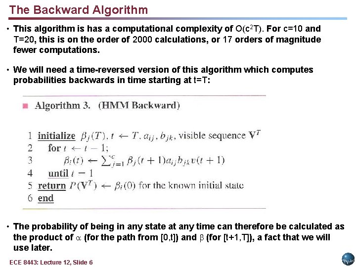
The Backward Algorithm • This algorithm is has a computational complexity of O(c 2 T). For c=10 and T=20, this is on the order of 2000 calculations, or 17 orders of magnitude fewer computations. • We will need a time-reversed version of this algorithm which computes probabilities backwards in time starting at t=T: • The probability of being in any state at any time can therefore be calculated as the product of (for the path from [0, t]) and (for [t+1, T]), a fact that we will use later. ECE 8443: Lecture 12, Slide 6

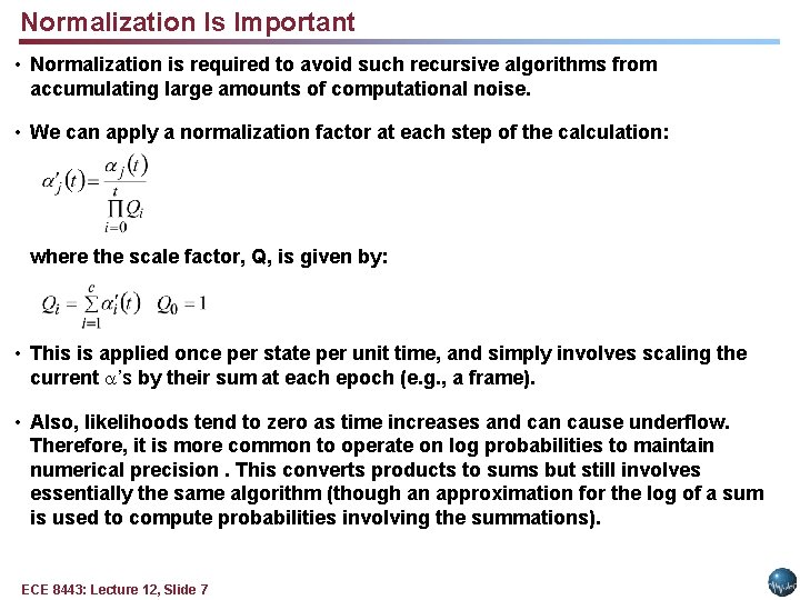
Normalization Is Important • Normalization is required to avoid such recursive algorithms from accumulating large amounts of computational noise. • We can apply a normalization factor at each step of the calculation: where the scale factor, Q, is given by: • This is applied once per state per unit time, and simply involves scaling the current ’s by their sum at each epoch (e. g. , a frame). • Also, likelihoods tend to zero as time increases and can cause underflow. Therefore, it is more common to operate on log probabilities to maintain numerical precision. This converts products to sums but still involves essentially the same algorithm (though an approximation for the log of a sum is used to compute probabilities involving the summations). ECE 8443: Lecture 12, Slide 7

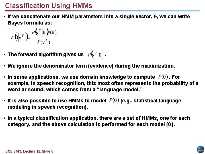
Classification Using HMMs • If we concatenate our HMM parameters into a single vector, , we can write Bayes formula as: • The forward algorithm gives us . • We ignore the denominator term (evidence) during the maximization. • In some applications, we use domain knowledge to compute. For example, in speech recognition, this most often represents the probability of a word or sound, which comes from a “language model. ” • It is also possible to use HMMs to modeling in speech recognition). (e. g. , statistical language • In a typical classification application, there a set of HMMs, one for each category, and the above calculation is performed for each model ( i). ECE 8443: Lecture 12, Slide 8

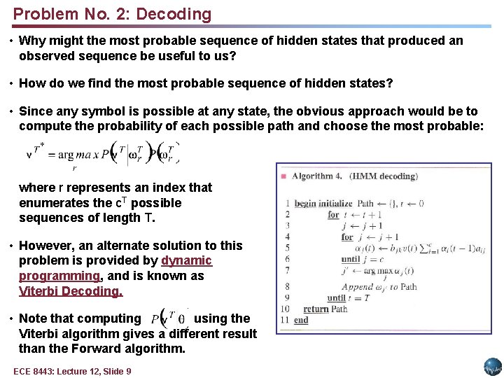
Problem No. 2: Decoding • Why might the most probable sequence of hidden states that produced an observed sequence be useful to us? • How do we find the most probable sequence of hidden states? • Since any symbol is possible at any state, the obvious approach would be to compute the probability of each possible path and choose the most probable: where r represents an index that enumerates the c. T possible sequences of length T. • However, an alternate solution to this problem is provided by dynamic programming, and is known as Viterbi Decoding. • Note that computing using the Viterbi algorithm gives a different result than the Forward algorithm. ECE 8443: Lecture 12, Slide 9

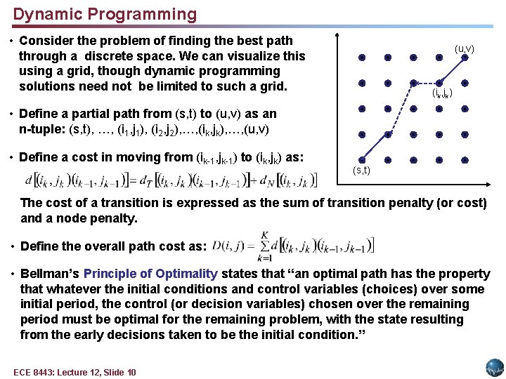
Dynamic Programming • Consider the problem of finding the best path through a discrete space. We can visualize this using a grid, though dynamic programming solutions need not be limited to such a grid. (u, v) (ik, jk) • Define a partial path from (s, t) to (u, v) as an n-tuple: (s, t), …, (i 1, j 1), (i 2, j 2), …, (ik, jk), …, (u, v) • Define a cost in moving from (ik-1, jk-1) to (ik, jk) as: (s, t) The cost of a transition is expressed as the sum of transition penalty (or cost) and a node penalty. • Define the overall path cost as: • Bellman’s Principle of Optimality states that “an optimal path has the property that whatever the initial conditions and control variables (choices) over some initial period, the control (or decision variables) chosen over the remaining period must be optimal for the remaining problem, with the state resulting from the early decisions taken to be the initial condition. ” ECE 8443: Lecture 12, Slide 10

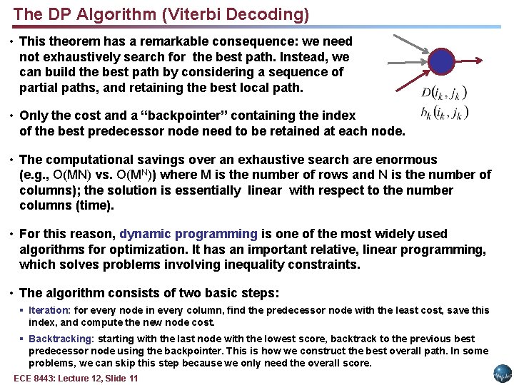
The DP Algorithm (Viterbi Decoding) • This theorem has a remarkable consequence: we need not exhaustively search for the best path. Instead, we can build the best path by considering a sequence of partial paths, and retaining the best local path. • Only the cost and a “backpointer” containing the index of the best predecessor node need to be retained at each node. • The computational savings over an exhaustive search are enormous (e. g. , O(MN) vs. O(MN)) where M is the number of rows and N is the number of columns); the solution is essentially linear with respect to the number columns (time). • For this reason, dynamic programming is one of the most widely used algorithms for optimization. It has an important relative, linear programming, which solves problems involving inequality constraints. • The algorithm consists of two basic steps: § Iteration: for every node in every column, find the predecessor node with the least cost, save this index, and compute the new node cost. § Backtracking: starting with the last node with the lowest score, backtrack to the previous best predecessor node using the backpointer. This is how we construct the best overall path. In some problems, we can skip this step because we only need the overall score. ECE 8443: Lecture 12, Slide 11

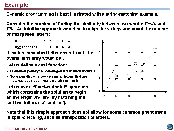
Example • Dynamic programming is best illustrated with a string-matching example. • Consider the problem of finding the similarity between two words: Pesto and Pita. An intuitive approach would be to align the strings and count the number of misspelled letters: Reference: P I ** t a Hypothesis: P e s o t If each mismatched letter costs 1 unit, the overall similarity would be 3. • Let us define a cost function: § Transition penalty: a non-diagonal transition incurs a penalty of 1 unit. § Node penalty: Any two dissimilar letters that are matched at a node incur a penalty of 1 unit. • Let us use a “fixed-endpoint” approach, which constrains the solution to begin an the origin and end by matching the last two letters (“a” and “o”). • Note that this simple approach does not allow for some common phenomena in spell-checking, such as transposition of letters. ECE 8443: Lecture 12, Slide 12

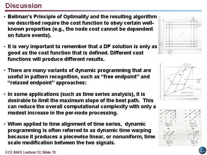
Discussion • Bellman’s Principle of Optimality and the resulting algorithm we described require the cost function to obey certain wellknown properties (e. g. , the node cost cannot be dependent on future events). • It is very important to remember that a DP solution is only as good as the cost function that is defined. Different cost functions will produce different results. • There are many variants of dynamic programming that are useful in pattern recognition, such as “free endpoint” and “relaxed endpoint” approaches: • In some applications (such as time series analysis), it is desirable to limit the maximum slope of the best path. This can reduce the overall computational complexity with only a modest increase in the per-node processing. • When applied to time alignment of time series, dynamic programming is often referred to as dynamic time warping because it produces a piecewise linear, or nonuniform, time scale modification between the two signals. ECE 8443: Lecture 12, Slide 13

Summary • Formally introduced a hidden Markov model. • Described three fundamental problems (evaluation, decoding, and training). • Derived general properties of the model. • Introduced the Forward Algorithm as a fast way to do evaluation. • Introduced the Viterbi Algorithm as a reasonable way to do decoding. • Introduced dynamic programming using a string matching example. Remaining issues: • Derive the reestimation equations using the EM Theorem so we can guarantee convergence. • Generalize the output distribution to a continuous distribution using a Gaussian mixture model. ECE 8443: Lecture 12, Slide 14