Particle Filters for Localization Abnormality Detection Dan Bryce

Particle Filters for Localization & Abnormality Detection Dan Bryce Markoviana Reading Group Sunday, October 24, 2021

Problems • • Position Tracking Global Localization Kidnapped Robot (Failure Recovery) Multi Robot Localization

Solution Technique • MCL – Monte Carlo Localization – Particle Filter + Model of Sensors + Model of Effectors • Need: – Bel(x 0) : Prior or initial belief --- x is position, heading – p(xt|xt-1, ut-1): effector model, u is control (e. g. turn, drive) – p(yt|xt): sensor model, y is sensor’s estimate of distance (e. g. laser range finder) – q: sampling distribution

p(xt|xt-1, ut-1) • Effector model is the convolution of 3 distributions – Robot kinematics model – Rotation noise – Translation Noise

Digression: the “action” input • Notice that the transition function now is p(xt|xt-1, ut-1)—it is dependent both on the previous state xt-1 and the action done- ut-1 • The actions are presumably chosen by the robot during a policy computation phase – If we are _tracking_ the robot (as against robot localizing itself), then we won’t have access to Ut-1 input. . • So, our filtering problem is really a “plan monitoring problem” • This brings up interesting questions about how to combine planning and filtering/monitoring. For example, if the Robot loses its bearings, it may want to shift from the policy it is executing to a “find-your-bearings” policy (such as try going to the nearest wall)

p(yt|xt) • Convolution of two distributions (Fig 19. 2) – Ideal noise free model of laser range finder – Mixture of noise variables • P(correct reading) convolved with Gaussian noise • P(max reading) • Random noise following exponential distribution

p(yt|xt)

Menkes’ question • Menkes asked why the distribution of particles in the top figure of 19. 4 does not look as if particles are uniformly distributed. • One explanation is that even if the robot starts with a uniform prior, within one iteration (of transitioning the particles through transfer function, and weighting/resampling w. r. t sensor model, they may already start to die out in regions that are completely inconsistent with sensor readings

q • q = p(xt|xt-1, ut-1)Bel(xt-1) (19. 2. 4) – Sampling from effector model and prior – Good if sensors are bad, bad if sensors are good • Approximates 19. 2. 5 – True posterior that reflects sensors • Assigned weights are proportional to p(yt|xt) (19. 2. 6) – Adjust sample to reflect sensor model

q’ • Previous q assumed sensors were very noisy and gave them less influence on samples • (19. 3. 7) samples from p(yt|xt) – Rely more on senors and less on prior belief and last control • Several variations on setting weights …

Digression: getting particles at the right place • There are two issues with the particles—getting them in the right place (e. g. right robot pose), and getting their weights. • If all the particles are in the wrong parts of the pose space (all of which are inconsistent with the current sensor information), they all will get 0 weights and become all useless • If at least some particles are in the right pose-space, they can get non-zero weight and prosper (as happens in the MCL-randomparticle idea) • The best would be to make all the particles be in the part of the space where the posterior probability is high – Since we don’t know the posterior distribution, we have to either sample them from the prior and transition function – OR sample from the sensor model (i. e. find the poses that have high P(y|x) value for the y value that the sensors are giving us.

Variation 1 • For each sample, draw a pair of samples, one from prior, one from sensor model (19. 3. 9) • Importance factor is proportional to (xit|ut i ) , x -1 t-1 • No need to transform sample sets into densities • Importance factor may be zero for many poses

Kd-trees • A kd-tree is a tree with the following properties – Each node represents a rectilinear region (faces aligned with axes) – Each node is associated with an axis aligned plane that cuts its region into two, and it has a child for each sub-region – The directions of the cutting planes alternate with depth • First cut perpendicular to x-axis, then perpendicular to y, then z and then back to x (some variations apparently ignore this rule) • Kd-trees generalize octrees by allowing splitting planes at variable positions – Note that cut planes in different sub-trees at the same level do not have to be the same

Kd-tree Example 4 6 1 10 8 2 11 3 13 2 4 12 5 8 9 5 1 3 7 9 6 10 7 11 12 13

Another kd-tree

Variation 2 • Forward Sampling + kd-trees (Fig. 19. 16) to approximate q’ = p(xt|d 0…t-1, ut-1) – Sample a set from Bel(xjt-1), then p(xjt|ut-1, xjt-1) to get p(xjt|d 0…t-1, ut-1) – Turn set into kd-tree (generalize poses) – Weight is proportional to xit probability in kdtree • Weight is proportional to p(xit|d 0…t-1, ut-1)

Variation 3 • Best of 1 and 3: large weights, no forward sampling – Turn Bel(xt-1) into kd-tree. – Sample xit from P(yt|xt) – Sample xit-1 from P(xit|ut-1, xt-1) – Set weight to the probability of xit-1 in kd-tree • Weight is proportional to (xit|ut-1)Bel(xit-1)

Mixture proposal • q: fails if sensors are accurate • q’: fails when sensors are not accurate • When in doubt use – (1 - )q + q’ – They used = 0. 1, and second method to compute weight for q’ (Fig 19. 11) 1000 particles 50 particles

Kidnapped Robot • MCL > MCL w/noise > Mixture MCL

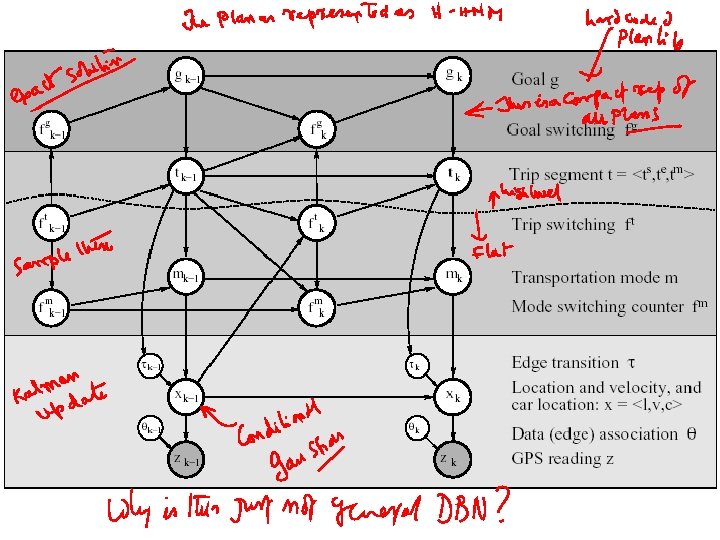
Learning and Inferring Transportation Routines • Engineering feat including many technologies – Abstract Hierarchical Markov Model • Represented as DBN • Inference with Rao-Blackwellised particle filter – EM – Error/Abnormality detection – Plan Recognition

H-HMM

RB-Filter Non-Gaussian Evidence

Tracking • Posterior • Sample – Sample high level discrete variables to get: – Then, predict gaussian filter of position with:

Tracking (cont’d) – Correction:

Goal and segment estimates • Do filtering as previously described (for nodes below line in graph), but allow lower nodes to be conditioned on upper nodes • For each filtered particle use exact inference to update gik and tik

Learning • Learn Structural (Flat) Model – Goals: EM for edge duration, then cluster – transfer points – count transitions in F/B pass • Learn Hierarchical transition probabilities – between goals, segments given goal, streets given segment

Detecting Errors • Can’t add all possible unknown goals and transfers to model • Instead use two trackers (combined with Bayes Factors) – First uses hierarchical model (fewer, costly particles) – Second uses flat model (more, cheap particles)

Comparison to Flat and 2 MM

Qns. . • In what sense is an AHMM a HMM rather than just a general DBN? • The issue of converting the agent plans into a compact AHMM—seems to make assumptions about the compactness of the set of behaviors the agent is likely to exhibit. – It seems as if the plan recognition problem at hand would have been quite easy in deterministic domains (since the agent is involved in only a few plans at most)

Combining plan synthesis and plan monitoring • We discussed about the possibility of hooking up the MCL style plan monitoring engine to a plan synthesis algorithm • Dan/Will said their simulator for Chitta’s class last year was a non-deterministic simulator (which doesn’t take likelihoods into account). – Would be nice to extend it • It would then be nice to interleave monitoring and replanning (when monitoring says that things are seriously afoul).