Particle Filters Application Examples Robot localization Robot mapping

Particle Filters

Application Examples • Robot localization • Robot mapping • Visual Tracking –e. g. human motion (body parts) • Prediction of (financial) time series –e. g. mapping gold price to stock price • Target recognition from single or multiple images • Guidance of missiles • Contour grouping • Nice video demos: http: //www. cs. washington. edu/ai/Mobile_Robotics/mcl/

2 nd Book Advert • • • Statistical Pattern Recognition Andrew Webb, DERA ISBN 0340741643, Paperback: 1999: £ 29. 99 Butterworth Heinemann • Contents: – Introduction to SPR, Estimation, Density estimation, Linear discriminant analysis, Nonlinear discriminant analysis - neural networks, Nonlinear discriminant analysis - statistical methods, Classification trees, Feature selction and extraction, Clustering, Additional topics, Measures of dissimilarity, Parameter estimation, Linear algebra, Data, Probability theory.
")
Homework • Implement all three particle filter algorithms SIS Particle Filter Algorithm (p. 27) Basic SIR Particle Filter algorithm (p. 39, 40) Generic SIR Particle Filter algorithm (p. 42) • and evaluate their performance on a problem of your choice. • Groups of two are allowed. • Submit a report and a ready to run Matlab code (with a script and the data). • Present a report to the class.

Particle Filters n n n Often control models are non-linear and noise is nongausian. We use particles to represent the distribution “Survival of the fittest” Motion model Observation model (=weight) Proposal distribution
")
Particle Filters SIS-R algorithm n Initialize particles randomly (Uniformly or according to prior knowledge) n At each time step: n Sequential importance sampling For each particle: n n Use motion model to predict new pose (sample from transition priors) Use observation model to assign a weight to each particle (posterior/proposal) Motion model Observation model (=weight) Proposal distribution
 n")
Particle Filters RE-SAMPLING n Initialize particles randomly (Uniformly or according to prior knowledge) n At each time step: n Sequential importance sampling Selection: n Resampling For each particle: n n Use motion model to predict new pose (sample from transition priors) Use observation model to assign a weight to each particle (posterior/proposal) Create A new set of equally weighted particles by sampling the distribution of the weighted particles produced in the previous step.

Example 1 of a Particle Filter Something is known

Particle Filters – Example 1

Particle Filters – Example 1 Use motion model to predict new pose (move each particle by sampling from the transition prior)
")
Particle Filters – Example 1 Use measurement model to compute weights (weight: observation probability)

Particle Filters – Example 1 Resample

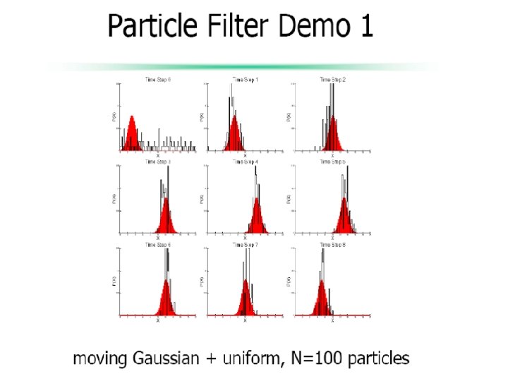
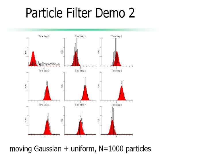
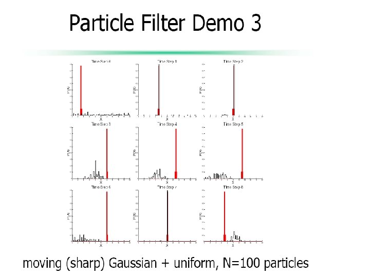
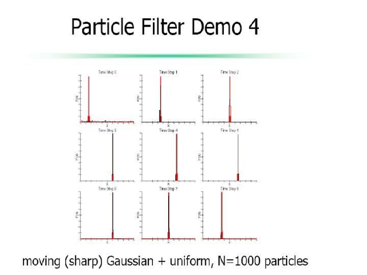
Example 2 of a Particle Filter Nothing is known

Particle Filters – Example 2 Initialize particles uniformly

Particle Filters – Example 2

Particle Filters – Example 2

Particle Filters – Example 2

Particle Filters – Example 2

Particle Filters – Example 2

Discussion of Continuous State Approaches Kalman Filters pluses ì Perform very accurately if the inputs are precise (performance is optimal with respect to any criterion in the linear case). ì Computational efficiency. minuses î Requirement that the initial state is known. î Inability to recover from catastrophic failures î Inability to track Multiple Hypotheses the state (Gaussians have only one mode)
 to operate")
Discussion of Discrete State Approaches Particle Filters ì Ability (to some degree) to operate even when its initial pose is unknown (start from uniform distribution). ì Ability to deal with noisy measurements. ì Ability to represent ambiguities (multi modal distributions). î Computational time scales heavily with the number of possible states (dimensionality of the grid, number of samples, size of the map). î Accuracy is limited by the size of the grid cells/number of particles-sampling method. î Required number of particles is unknown

27

28

Sources Paul E. Rybski Haris Baltzakis • 29

PR Virtual Architecture with Kalman Filters 1. Sensor records samples 2. Image processing step extracts specific features – Target size, vertical position, horizontal position, target bearing, elevation, etc. 3. Kalman filters extract sensor noise 4. Results are sent to a central location to be displayed
- Slides: 30