Part 3 Linear Programming 3 3 Theoretical Analysis

Part 3 Linear Programming 3. 3 Theoretical Analysis

Matrix Form of the Linear Programming Problem

Feasible Solution in Matrix Form

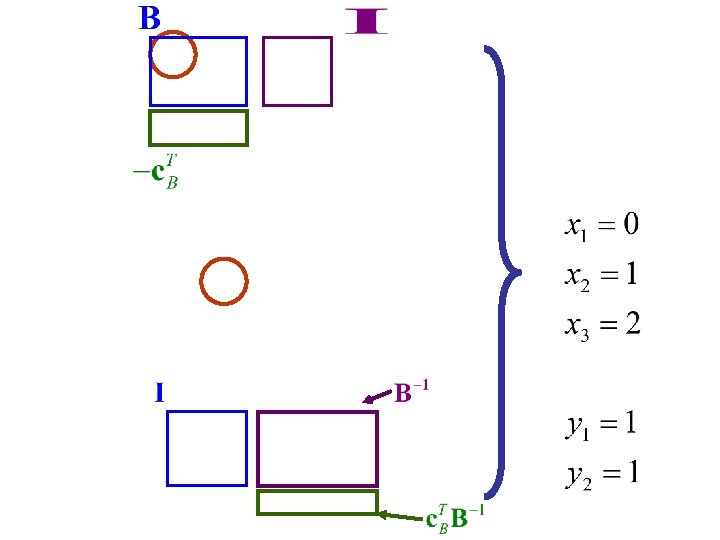
Tableau in Matrix Form (without the objective column)

Criteria for Determining A Minimum Feasible Solution

Theorem (Improvement of Basic Feasible Solution) • Given a non-degenerate basic feasible solution with corresponding objective function f 0, suppose for some j there holds cj-fj<0. Then there is a feasible solution with objective value f<f 0. • If the column aj can be substituted for some vector in the original basis to yield a new basic feasible solution, this new solution will have f<f 0. • If aj cannot be substituted to yield a basic feasible solution, then the solution set K is unbounded and the objective function can be made arbitrarily small (negative) toward minus infinity.

Optimality Condition for a Minimum! •

Symmetric Form of Duality (1)

Symmetric Form of Duality (2) •

Alternative Form of Duality

Example Batch Reactor B Batch Reactor A Batch Reactor C Raw materials R 1, R 2, R 3, R 4 Products P 1, P 2, P 3, P 4 P 1 P 2 P 3 P 4 capacity time A 1. 5 1. 0 2. 4 1. 0 2000 B 1. 0 5. 0 1. 0 3. 5 8000 C 1. 5 3. 0 3. 5 1. 0 5000 profit /batch $5. 24 $7. 30 $8. 34 $4. 18 time/batch

Example: Primal Problem

Example: Dual Problem

Property 1 For any feasible solution to the primal problem and any feasible solution to the dual problem, the value of the primal objective function being maximized is always equal to or less than the value of the dual objective function being minimized.

Proof

Property 2

Proof

Duality Theorem If either the primal or dual problem has a finite optimal solution, so does the other, and the corresponding values of objective functions are equal. If either problem has an unbounded objective, the other problem has no feasible solution.

Alternative Form of Duality

Additional Insights Shadow Prices!

Matrix Form of the Linear Programming Problem

Feasible Solution in Matrix Form

Tableau in Matrix Form (without the objective column!)

Relations associated with the Optimal Feasible Solution of the Primal (Minimization) Problem This is the optimality condition of the primal minimization problem! Property 2 is satisfied!

Example PRIMAL DUAL

Tableau in Matrix Form of Primal Problem

Example: The Primal Diet Problem •

Primal Formulation

Alternative Form of Duality

The Dual Diet Problem •

Dual Formulation

Shadow Prices How does the minimum cost in the primal problem change if we change the right hand side b (lower limits of nutrient j)? If the changes are small, then the corner which was optimal remains optimal, i. e. – The choice of basic variables does not change. – At the end of simplex method, the corresponding m columns of A make up the basis matrix B.