Ch 7 LINEAR PROGRAMMING Linear programming 1 is

Ch 7 LINEAR PROGRAMMING Linear programming 1 is a mathematical technique that enables a decision maker to arrive at the optimal solution to problems involving the allocation of scarce resources. Typically, many economic and technical problems involve maximization or minimization of a certain objective subject to some restrictions. 1 During World War II US army began to formulate certain linear optimization problems. Their solutions were called plans or programs. Today important application areas include airline crew scheduling, shipping or telecommunication networks, oil refining and blending, and stock and bond portfolio selection. 1

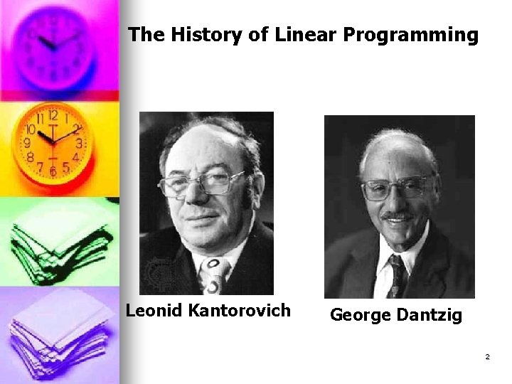
The History of Linear Programming Leonid Kantorovich George Dantzig 2

Programming problems, in general, are concerned with the use or allocation of scarce resources - labor, materials, machines, and capital - in the ”best” possible manner so that costs are minimized or profits maximized. In using the term ”best possible” it is implied that some choice or set of alternative courses of actions is available for making the decision. 3

Typical Applications of Linear Programming 1. A manufacturer wants to develop a production schedule and inventory policy that will satisfy sales demand in future periods and same time minimize the total production and inventory cost. 2. A financial analyst must select an investment portfolio from a variety of stock and bond investment alternatives. He would like to establish the portfolio that maximizes the return on investment. 4

Typical Applications of Linear Programming continued 3. A marketing manager wants to determine how best to allocate a fixed advertising budget among alternative advertising media such as radio, TV, newspaper, and magazines. The goal is to maximize advertising effectiveness. 4. A company has warehouses in a number of locations throughout the country. For a set of customer demands for its products, the company would like to determine how much each warehouse should ship to each customer so that the total transportation costs are minimized. 5

Constructing Linear Programming Next we list what is required in order Models to construct a linear programming model: 1. Objective Function. There must be an objective (or goal or target) the firm or organization wants to achieve. For example, maximize dollar profits, minimize dollar cost, maximize total number of expected potential customers, minimize total time used, and so forth. 6

Constructing Linear Programming Models continued 2. Restrictions and Decisions. There must be alternative courses of action or decisions, one of which will achieve the objective. 3. Linear Objective Function and Linear Constraints. We must be able to express the decision problem incorporating the objective and restrictions on the decisions using only linear equations and linear inequalities. i. e. , we must be able to state the problem as a linear programming model. 7

Economic Significance of Linearity The simplifying assumption of linearity causes some problems: 1. In profit-maximizing production problem linearity of the objective function implies constant profit rate per unit as output increases; this means a) that the selling price is constant; and 8

b) that average variable cost is constant; the law of diminishing returns does not influence the production process, and input prices are constant perfect competition in output and input markets 2. Linear resource constraints imply constant combination of inputs; this means constant returns to scale. 9

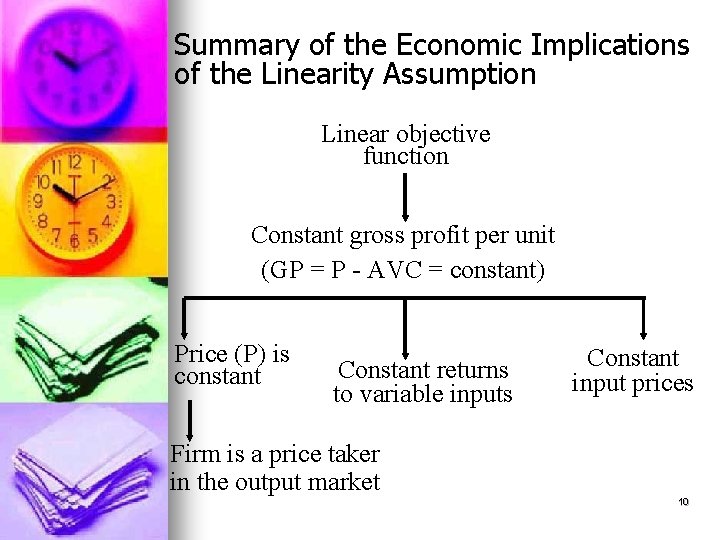
Summary of the Economic Implications of the Linearity Assumption Linear objective function Constant gross profit per unit (GP = P - AVC = constant) Price (P) is constant Constant returns to variable inputs Constant input prices Firm is a price taker in the output market 10

The three basic steps in constructing a linear programming model: Step I Identify the unknown variables to be determined (decision variables), and represent them in terms of algebraic symbols. 11

Step II Identify all the restrictions or constraints in the problem and express them as linear equations or inequalities which are linear functions of the unknown variables. 12

Step III Identify the objective or criterion and represent it as a linear function of the decision variables, which is to be maximized or minimized. 13

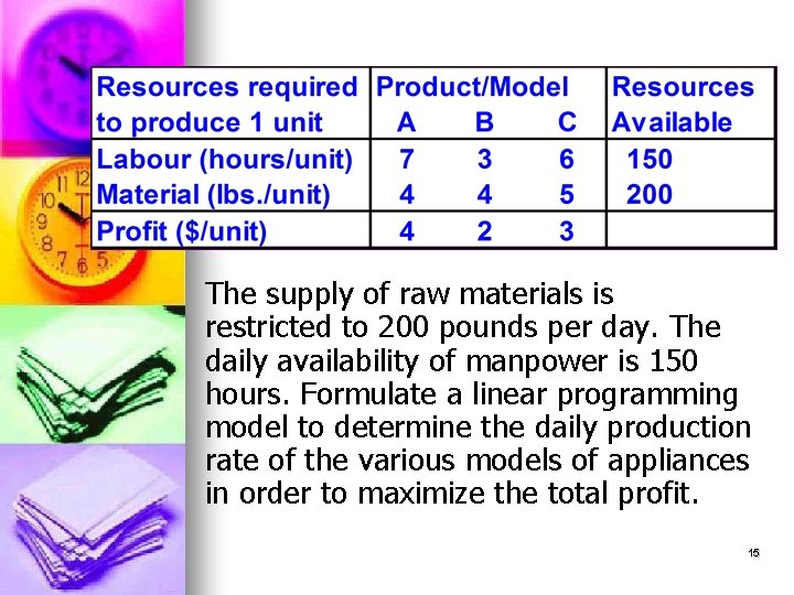
Example 1 Product-Mix Problem The Handy-Dandy Company wishes to schedule the production of a kitchen appliance which requires two resources – labor and material. The company is considering three different models of this appliance and its engineering department has furnished the following data: 14

The supply of raw materials is restricted to 200 pounds per day. The daily availability of manpower is 150 hours. Formulate a linear programming model to determine the daily production rate of the various models of appliances in order to maximize the total profit. 15

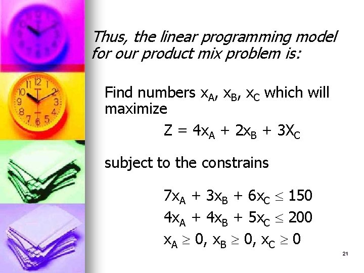
Step I Identify the Decision Variables. The unknown activities to be determined are the daily rate of production for the three models (A, B, C) in order to maximize the total profit. Representing them by algebraic symbols, x. A = daily production of model A x. B = daily production of model B x. C = daily production of model C 16

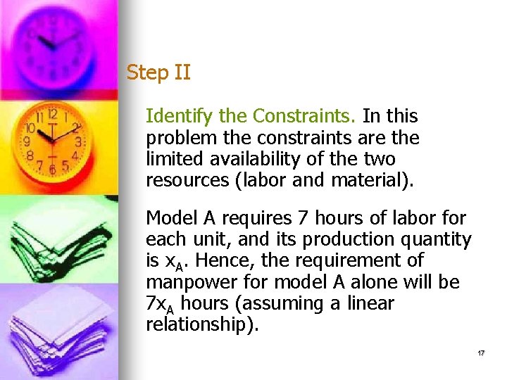
Step II Identify the Constraints. In this problem the constraints are the limited availability of the two resources (labor and material). Model A requires 7 hours of labor for each unit, and its production quantity is x. A. Hence, the requirement of manpower for model A alone will be 7 x. A hours (assuming a linear relationship). 17

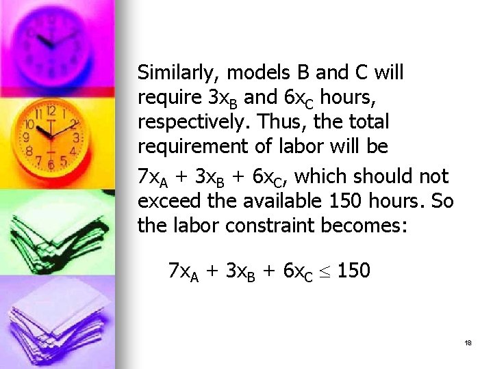
Similarly, models B and C will require 3 x. B and 6 x. C hours, respectively. Thus, the total requirement of labor will be 7 x. A + 3 x. B + 6 x. C, which should not exceed the available 150 hours. So the labor constraint becomes: 7 x. A + 3 x. B + 6 x. C 150 18

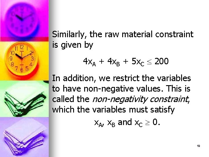
Similarly, the raw material constraint is given by 4 x. A + 4 x. B + 5 x. C 200 In addition, we restrict the variables to have non-negative values. This is called the non-negativity constraint, which the variables must satisfy x. A, x. B and x. C 0. 19

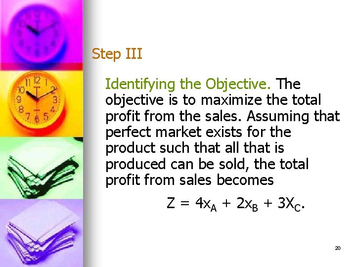
Step III Identifying the Objective. The objective is to maximize the total profit from the sales. Assuming that perfect market exists for the product such that all that is produced can be sold, the total profit from sales becomes Z = 4 x. A + 2 x. B + 3 XC. 20

Thus, the linear programming model for our product mix problem is: Find numbers x. A, x. B, x. C which will maximize Z = 4 x. A + 2 x. B + 3 XC subject to the constrains 7 x. A + 3 x. B + 6 x. C 150 4 x. A + 4 x. B + 5 x. C 200 x. A 0, x. B 0, x. C 0 21

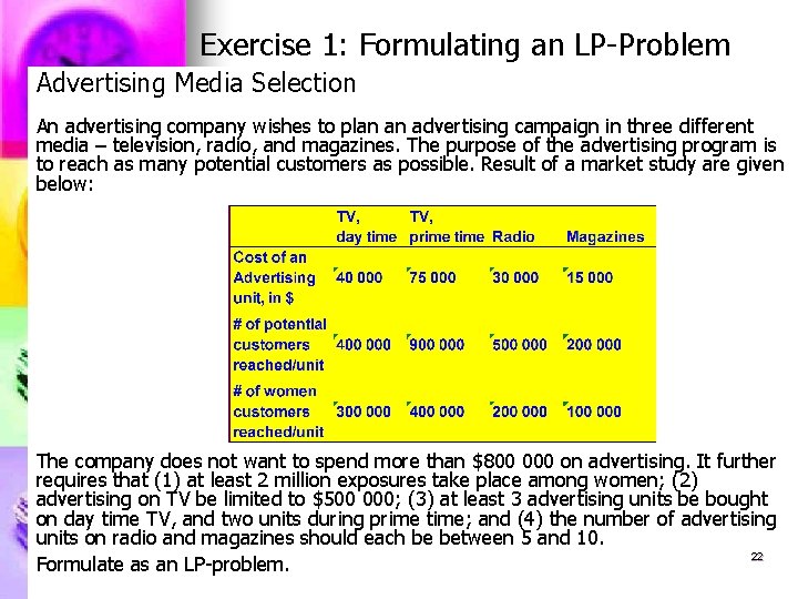
Exercise 1: Formulating an LP-Problem Advertising Media Selection An advertising company wishes to plan an advertising campaign in three different media – television, radio, and magazines. The purpose of the advertising program is to reach as many potential customers as possible. Result of a market study are given below: The company does not want to spend more than $800 000 on advertising. It further requires that (1) at least 2 million exposures take place among women; (2) advertising on TV be limited to $500 000; (3) at least 3 advertising units be bought on day time TV, and two units during prime time; and (4) the number of advertising units on radio and magazines should each be between 5 and 10. 22 Formulate as an LP-problem.

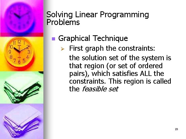
Solving Linear Programming Problems n Graphical Technique Ø First graph the constraints: the solution set of the system is that region (or set of ordered pairs), which satisfies ALL the constraints. This region is called the feasible set 23

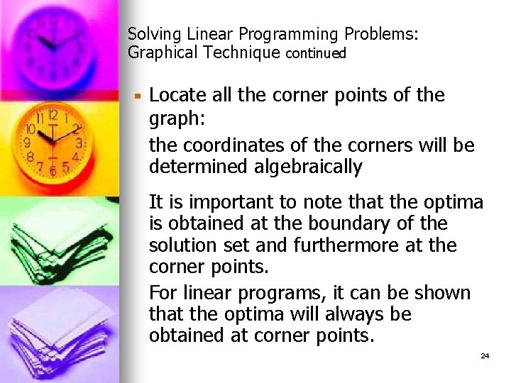
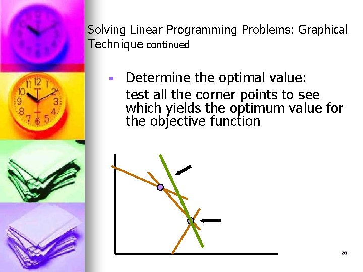
Solving Linear Programming Problems: Graphical Technique continued ￭ Locate all the corner points of the graph: the coordinates of the corners will be determined algebraically It is important to note that the optima is obtained at the boundary of the solution set and furthermore at the corner points. For linear programs, it can be shown that the optima will always be obtained at corner points. 24

Solving Linear Programming Problems: Graphical Technique continued ￭ Determine the optimal value: test all the corner points to see which yields the optimum value for the objective function Objective function Feasible set Optimum 25

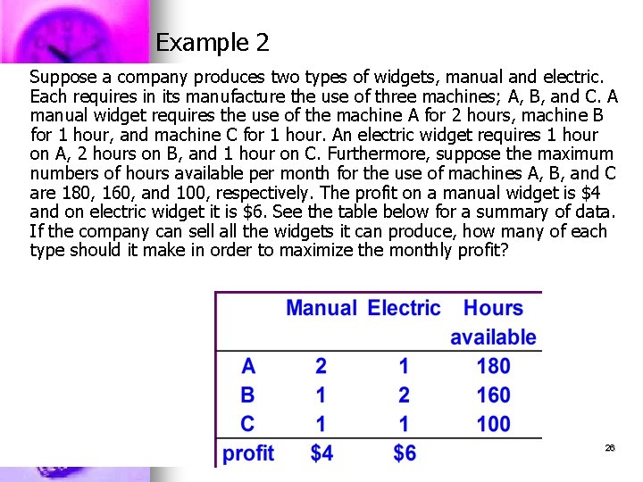
Example 2 Suppose a company produces two types of widgets, manual and electric. Each requires in its manufacture the use of three machines; A, B, and C. A manual widget requires the use of the machine A for 2 hours, machine B for 1 hour, and machine C for 1 hour. An electric widget requires 1 hour on A, 2 hours on B, and 1 hour on C. Furthermore, suppose the maximum numbers of hours available per month for the use of machines A, B, and C are 180, 160, and 100, respectively. The profit on a manual widget is $4 and on electric widget it is $6. See the table below for a summary of data. If the company can sell all the widgets it can produce, how many of each type should it make in order to maximize the monthly profit? 26

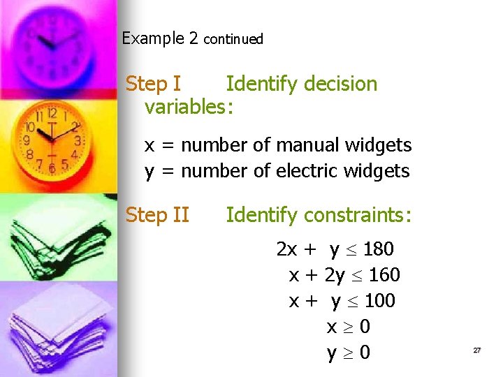
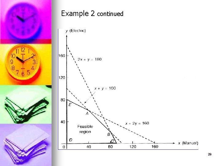
Example 2 continued Step I Identify decision variables: x = number of manual widgets y = number of electric widgets Step II Identify constraints: 2 x + y 180 x + 2 y 160 x + y 100 x 0 y 0 27

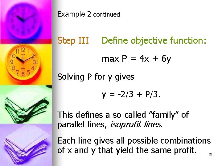
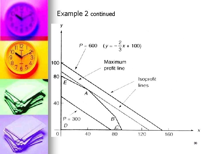
Example 2 continued Step III Define objective function: max P = 4 x + 6 y Solving P for y gives y = -2/3 + P/3. This defines a so-called ”family” of parallel lines, isoprofit lines. Each line gives all possible combinations of x and y that yield the same profit. 28

Example 2 continued 29

Example 2 continued 30

Exercise 2: Solving an LP-problem: A California vintner has available 660 lbs of Cabernet Sauvignon (CS) grapes, 1860 lbs of Pinot Noir (PN) grapes, and 2100 lbs of Barbera (B) grapes. The vintner makes a Pinot Noir (PN) wine, which contains 20% CS, 60% PN, and 20% B grapes and sells $3 a bottle, and a Barbera (B) wine, which contains 10% CS, 20% PN, and 70% B grapes and sells for $2 a bottle. Assuming each bottle of wine requires 3 lbs of grapes, determine how many bottles of each type of wine should be produced to maximize income. 31

Solving an LP-problem continued: n Algebraic Technique Ø Ø Ø The graphical method solving linear programming problems can be used for problems with two variables (with some difficulty three) However, for problems were the number of variables might run into hundreds or thousands, algebraic techniques must be used The simplex method, with the aid of the computer, can solve these problems 32

As with the graphical procedure, the simplex method finds the optimal corner-point solution of the set of feasible solutions. Regardless of the number of decision variables and regardless of the number of constraints, the simplex method uses the key property of a linear programming problem, which is: 33

n A linear programming problem always has an optimal solution occurring at a corner-point solution Simplex method begins with a feasible solution and tests whether or not it is optimum. If not optimum, the method proceeds to a better solution. 34

Solution of a maximum-type linear programming problem by the simplex algorithm involves the following steps: 1. Adding slack variables to convert the inequalities into equations In the case of less-than-or-equal-to constraints, slack variables are used to increase the left-hand side to equal the right-hand side limits of the constraint conditions. 35

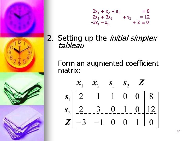
Example: max Z = 3 x 1 + x 2 st. 2 x 1 + x 2 8 2 x 1 + 3 x 2 12 adding slacks and rewriting the object row: 2 x 1 + x 2 + s 1 =8 2 x 1 + 3 x 2 + s 2 = 12 -3 x 1 – x 2 +Z =0 where x 1, x 2, s 1 and s 2 are non-negative. 36

2 x 1 + x 2 + s 1 =8 2 x 1 + 3 x 2 + s 2 = 12 -3 x 1 – x 2 +Z=0 2. Setting up the initial simplex tableau Form an augmented coefficient matrix: 37

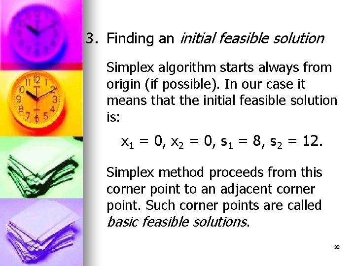
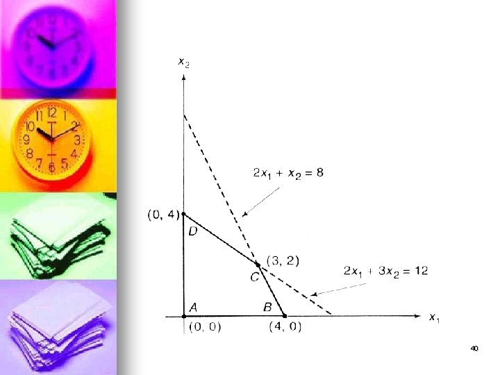
3. Finding an initial feasible solution Simplex algorithm starts always from origin (if possible). In our case it means that the initial feasible solution is: x 1 = 0, x 2 = 0, s 1 = 8, s 2 = 12. Simplex method proceeds from this corner point to an adjacent corner point. Such corner points are called basic feasible solutions. 38

4. Introducing basic and nonbasic variables as the natural way to express basic feasible solutions For any basic feasible solution (B. F. S. ), the variables held zero are called nonbasic variables and the other are called basic variables. Moving form one B. F. S. to another means that one basic variable (we call it a departing or exiting variable) becomes nonbasic and a nonbasic variable (entering variable) becomes a basic variable. 39

40

5. Choosing the proper pivot element to advance the solution and maintain the non-negativity of all variables How to decide which variable to make basic and which nonbasic (in other words in which direction to move from the current B. F. S. )? 41

The natural direction is the one in which the value of the objective function increases the most: If in Z = 3 x 1 + x 2, x 1 is allowed to become basic, x 2 remains at 0 and Z = 3 x 1; thus for each one-unit increase in x 1, Z increases by 3 units. On the other hand, if x 2 is allowed to become basic, Z will increase only by one unit if x 2 is increased by one unit. This is one way to determine the pivot column. 42

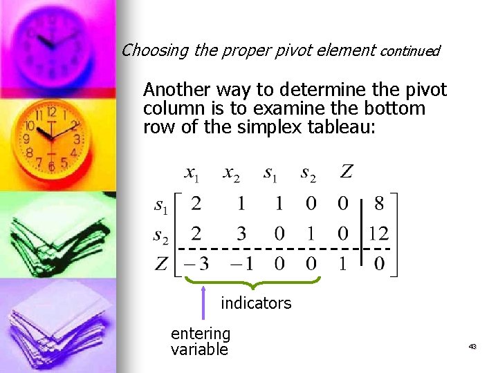
Choosing the proper pivot element continued Another way to determine the pivot column is to examine the bottom row of the simplex tableau: indicators entering variable 43

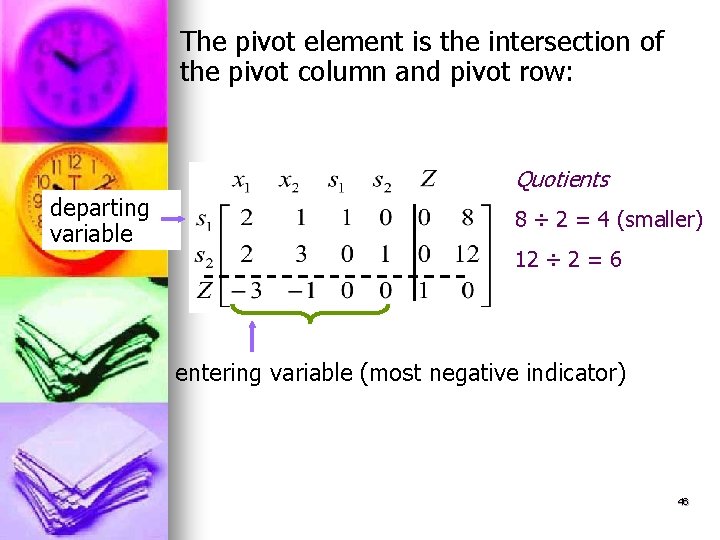
The bottom row entries to the left of the vertical line are called indicators. We choose the column with the most negative indicator as the pivot column. Having chosen the pivot column, we must now determine the pivot row in order to know which element in our simplex tableau is the pivoting element. 44

For that purpose we divide the right hand side entries of the simplex tableau by corresponding entries of the pivot column. Of the resulting quotients we choose the smallest (minimum quotient). So the pivot element is the intersection of the pivot column and pivot row. 45

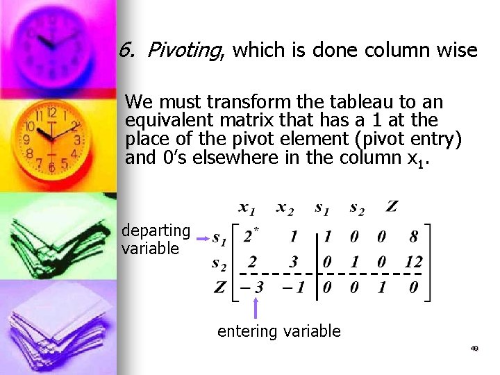
The pivot element is the intersection of the pivot column and pivot row: departing variable Quotients 8 ÷ 2 = 4 (smaller) 12 ÷ 2 = 6 entering variable (most negative indicator) 46

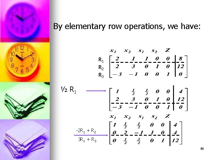
Since x 1 and s 2 will be the basic variables in our new B. F. S, it would be convenient to change our previous tableau by elementary row operations into a form where the values of x 1, s 2, and Z can be read off with ease just as in the initial basic solution. 47

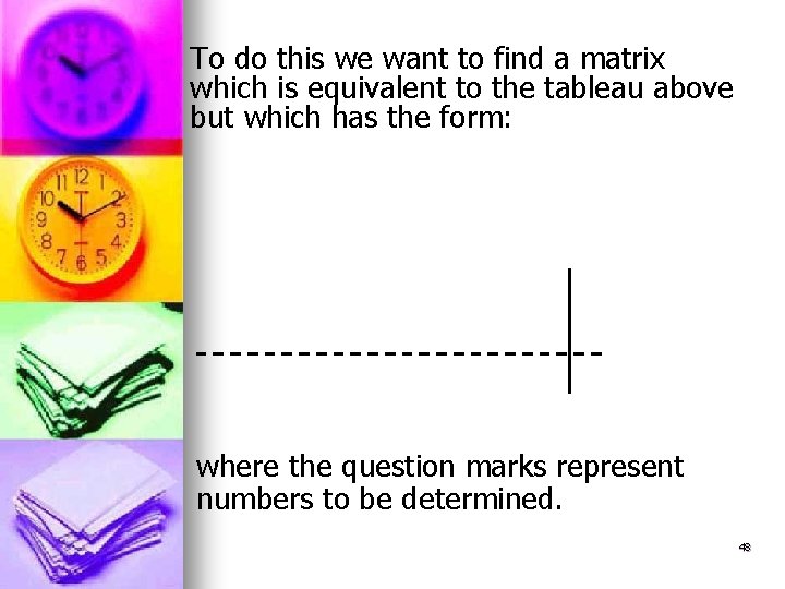
To do this we want to find a matrix which is equivalent to the tableau above but which has the form: where the question marks represent numbers to be determined. 48

6. Pivoting, which is done column wise We must transform the tableau to an equivalent matrix that has a 1 at the place of the pivot element (pivot entry) and 0’s elsewhere in the column x 1. departing variable entering variable 49

By elementary row operations, we have: R 1 R 2 R 3 ½ R 1 -2 R 1 + R 2 3 R 1 + R 3 50

7. Continuing and recognizing when the algorithm terminates. General termination rule: all values in the indicator row are non-negative. 51

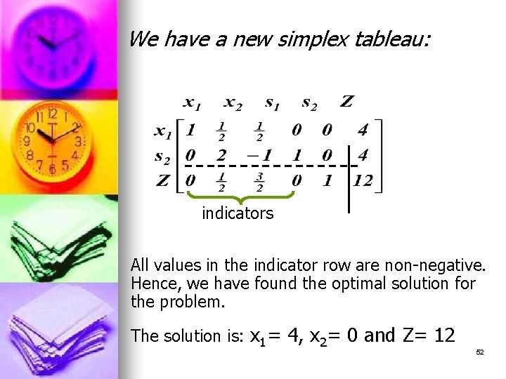
We have a new simplex tableau: indicators All values in the indicator row are non-negative. Hence, we have found the optimal solution for the problem. The solution is: x 1= 4, x 2= 0 and Z= 12 52