Parametrizations in Data Assimilation ECMWF Training Course 29

Parametrizations in Data Assimilation ECMWF Training Course 29 March 2017 Philippe Lopez Physical Processes Group, Research Department, ECMWF (Room 002)

Parametrizations in Data Assimilation • Introduction • Why are physical parametrizations needed in data assimilation? • Tangent-linear and adjoint coding • Issues related to physical parametrizations in data assimilation • Physical parametrizations in ECMWF’s current 4 D-Var system • Examples of applications • Summary and conclusions

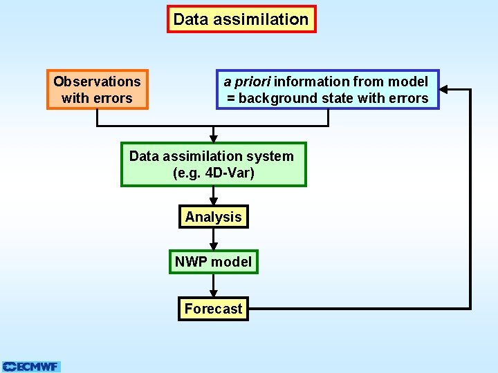
Data assimilation Observations with errors a priori information from model = background state with errors Data assimilation system (e. g. 4 D-Var) Analysis NWP model Forecast

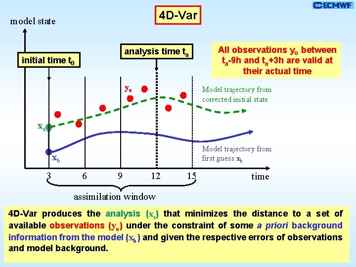
4 D-Var model state analysis time ta initial time t 0 yo All observations yo between ta-9 h and ta+3 h are valid at their actual time Model trajectory from corrected initial state xa Model trajectory from first guess xb xb 3 6 9 12 15 time assimilation window 4 D-Var produces the analysis (xa) that minimizes the distance to a set of available observations (yo) under the constraint of some a priori background information from the model (xb) and given the respective errors of observations and model background.

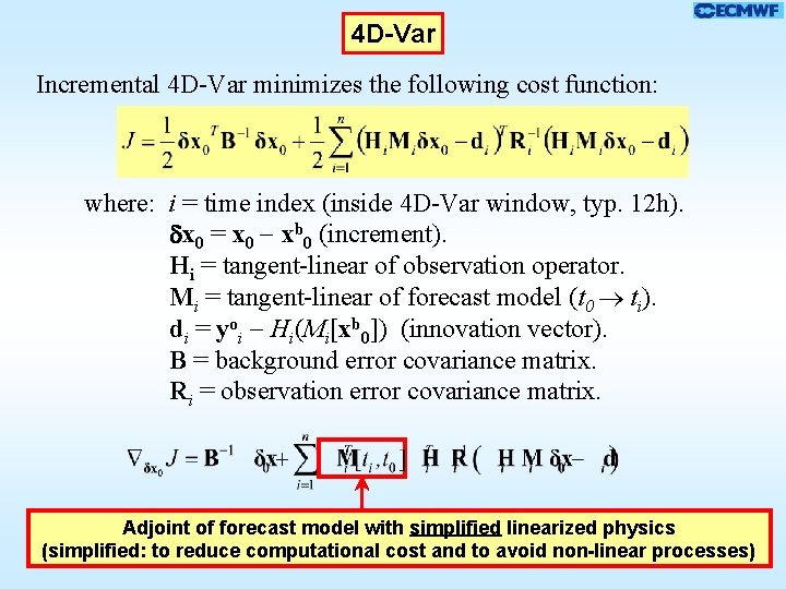
4 D-Var Incremental 4 D-Var minimizes the following cost function: where: i = time index (inside 4 D-Var window, typ. 12 h). x 0 = x 0 xb 0 (increment). Hi = tangent-linear of observation operator. Mi = tangent-linear of forecast model (t 0 ti). di = yoi Hi(Mi[xb 0]) (innovation vector). B = background error covariance matrix. Ri = observation error covariance matrix. Adjoint of forecast model with simplified linearized physics (simplified: to reduce computational cost and to avoid non-linear processes)

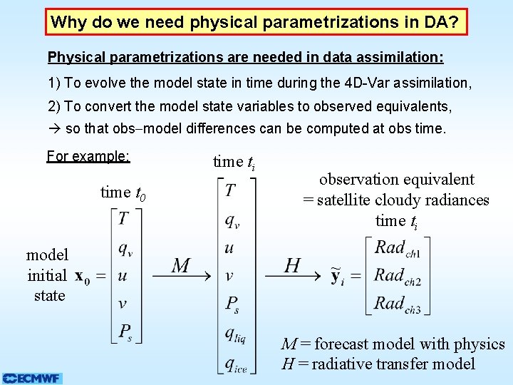
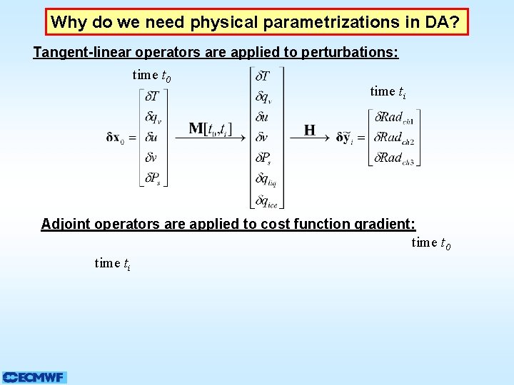
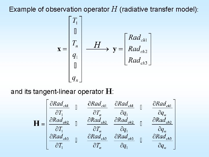
Why do we need physical parametrizations in DA? Physical parametrizations are needed in data assimilation: 1) To evolve the model state in time during the 4 D-Var assimilation, 2) To convert the model state variables to observed equivalents, so that obs model differences can be computed at obs time. For example: time t 0 time ti observation equivalent = satellite cloudy radiances time ti model initial state M = forecast model with physics H = radiative transfer model

Why do we need physical parametrizations in DA? Tangent-linear operators are applied to perturbations: time t 0 time ti Adjoint operators are applied to cost function gradient: time t 0 time ti

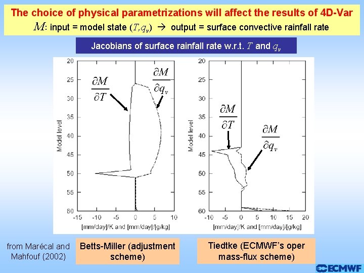
The choice of physical parametrizations will affect the results of 4 D-Var M: input = model state (T, qv) output = surface convective rainfall rate Jacobians of surface rainfall rate w. r. t. T and qv from Marécal and Mahfouf (2002) Betts-Miller (adjustment scheme) Tiedtke (ECMWF’s oper mass-flux scheme)

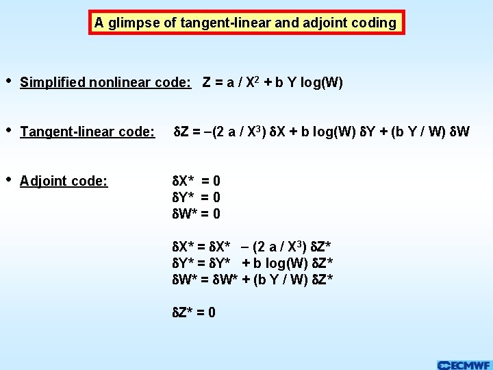
A glimpse of tangent-linear and adjoint coding • Simplified nonlinear code: Z = a / X 2 + b Y log(W) • Tangent-linear code: Z = (2 a / X 3) X + b log(W) Y + (b Y / W) W • Adjoint code: X* = 0 Y* = 0 W* = 0 X* = X* (2 a / X 3) Z* Y* = Y* + b log(W) Z* W* = W* + (b Y / W) Z* Z* = 0

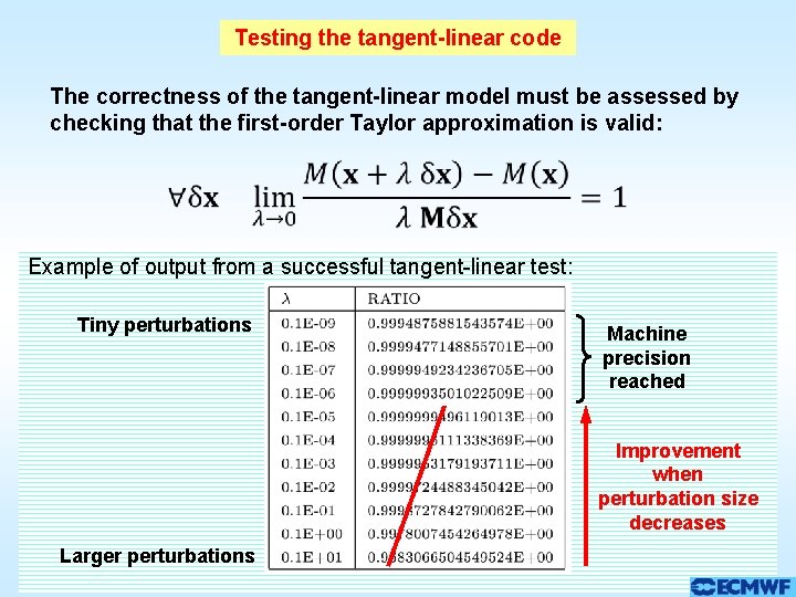
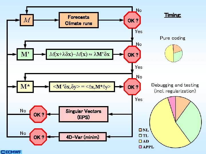
Testing the tangent-linear code The correctness of the tangent-linear model must be assessed by checking that the first-order Taylor approximation is valid: Example of output from a successful tangent-linear test: Tiny perturbations Machine precision reached Improvement when perturbation size decreases Larger perturbations

Testing the adjoint code The correctness of the adjoint model needs to be assessed by checking that it satisfies the mathematical relationship: where M is the tangent-linear model and MT is the adjoint model. Example of output from a successful adjoint test: <M x, y> = 0. 13765102625164 E-01 < x, MT y> = 0. 13765102625168 E-01 The difference is 11. 351 times the zero of the machine The adjoint test should be correct at the level of machine precision (typ. 13 to 15 digits for the entire model). Otherwise there must be a bug in the code!

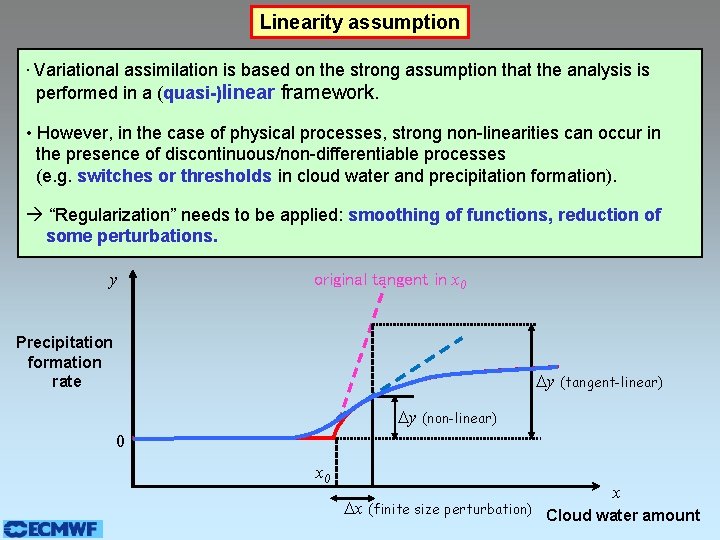
Linearity assumption • Variational assimilation is based on the strong assumption that the analysis is performed in a (quasi-)linear framework. • However, in the case of physical processes, strong non-linearities can occur in the presence of discontinuous/non-differentiable processes (e. g. switches or thresholds in cloud water and precipitation formation). “Regularization” needs to be applied: smoothing of functions, reduction of some perturbations. y original tangent in x 0 Precipitation formation rate Dy (tangent-linear) Dy (non-linear) 0 x Dx (finite size perturbation) Cloud water amount

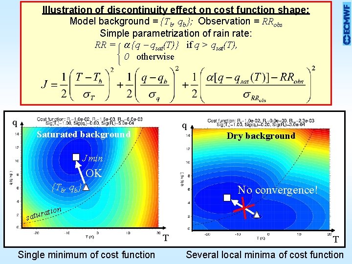
Illustration of discontinuity effect on cost function shape: Model background = {Tb, qb}; Observation = RRobs Simple parametrization of rain rate: RR = {q qsat(T)} if q > qsat(T), 0 otherwise q q Saturated background Dry background J min OK {Tb, qb} No convergence! on ati satur T Single minimum of cost function T Several local minima of cost function

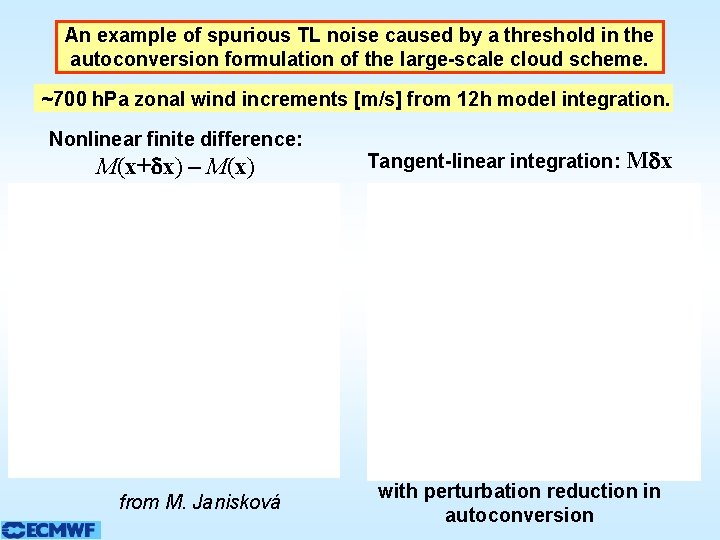
An example of spurious TL noise caused by a threshold in the autoconversion formulation of the large-scale cloud scheme. ~700 h. Pa zonal wind increments [m/s] from 12 h model integration. Nonlinear finite difference: M(x+ x) – M(x) from M. Janisková Tangent-linear integration: M x with perturbation reduction in autoconversion

No Forecasts Climate runs M Timing: OK ? Yes Pure coding No M’ M(x+ x) M(x) M’ x OK ? Yes No M* <M’ x, y> = < x, M* y> OK ? Yes No No OK ? Singular Vectors (EPS) OK ? 4 D-Var (minim) Debugging and testing (incl. regularization)

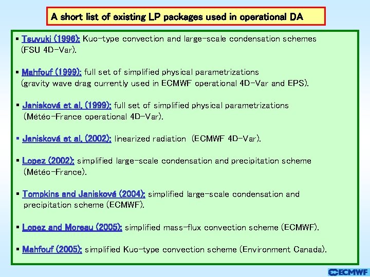
A short list of existing LP packages used in operational DA § Tsuyuki (1996): Kuo-type convection and large-scale condensation schemes (FSU 4 D-Var). § Mahfouf (1999): full set of simplified physical parametrizations (gravity wave drag currently used in ECMWF operational 4 D-Var and EPS). § Janisková et al. (1999): full set of simplified physical parametrizations (Météo-France operational 4 D-Var). § Janisková et al. (2002): linearized radiation (ECMWF 4 D-Var). § Lopez (2002): simplified large-scale condensation and precipitation scheme (Météo-France). § Tompkins and Janisková (2004): simplified large-scale condensation and precipitation scheme (ECMWF). § Lopez and Moreau (2005): simplified mass-flux convection scheme (ECMWF). § Mahfouf (2005): simplified Kuo-type convection scheme (Environment Canada).

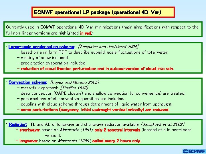
ECMWF operational LP package (operational 4 D-Var) Currently used in ECMWF operational 4 D-Var minimizations (main simplifications with respect to the full non-linear versions are highlighted in red): • Large-scale condensation scheme: [Tompkins and Janisková 2004] - based on a uniform PDF to describe subgrid-scale fluctuations of total water. - melting of snow included. - precipitation evaporation included. - reduction of cloud fraction perturbation and in autoconversion of cloud into rain. • Convection scheme: [Lopez and Moreau 2005] - mass-flux approach [Tiedtke 1989]. - deep convection (CAPE closure) and shallow convection (q-convergence) are treated. - perturbations of all convective quantities are included. - coupling with cloud scheme through detrainment of liquid water from updraught. - some perturbations (buoyancy, initial updraught vertical velocity) are reduced. • Radiation: TL and AD of longwave and shortwave radiation available [Janisková et al. 2002] - shortwave: based on Morcrette (1991), only 2 spectral intervals (instead of 6 in non-linear version). - longwave: based on Morcrette (1989), called every 2 hours only.

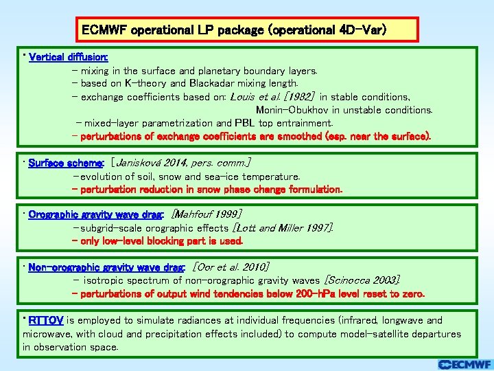
ECMWF operational LP package (operational 4 D-Var) • Vertical diffusion: - mixing in the surface and planetary boundary layers. - based on K-theory and Blackadar mixing length. - exchange coefficients based on: Louis et al. [1982] in stable conditions, Monin-Obukhov in unstable conditions. - mixed-layer parametrization and PBL top entrainment. - perturbations of exchange coefficients are smoothed (esp. near the surface). • Surface scheme: [Janisková 2014, pers. comm. ] - evolution of soil, snow and sea-ice temperature. - perturbation reduction in snow phase change formulation. • Orographic gravity wave drag: [Mahfouf 1999] - subgrid-scale orographic effects [Lott and Miller 1997]. - only low-level blocking part is used. • Non-orographic gravity wave drag: [Oor et al. 2010] - isotropic spectrum of non-orographic gravity waves [Scinocca 2003]. - perturbations of output wind tendencies below 200 -h. Pa level reset to zero. • RTTOV is employed to simulate radiances at individual frequencies (infrared, longwave and microwave, with cloud and precipitation effects included) to compute model–satellite departures in observation space.

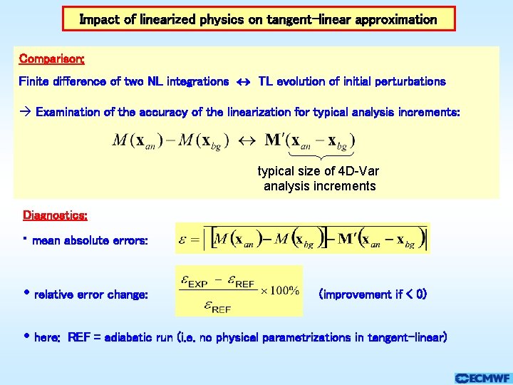
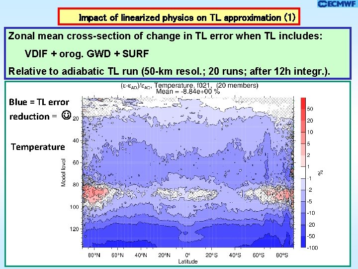
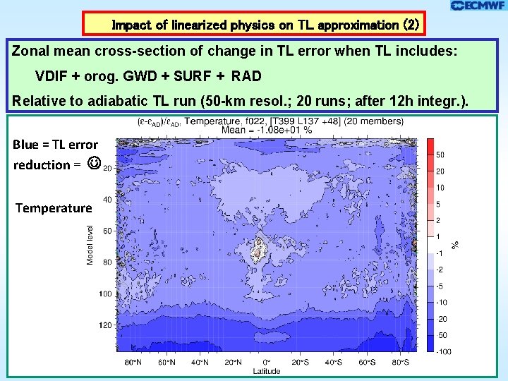
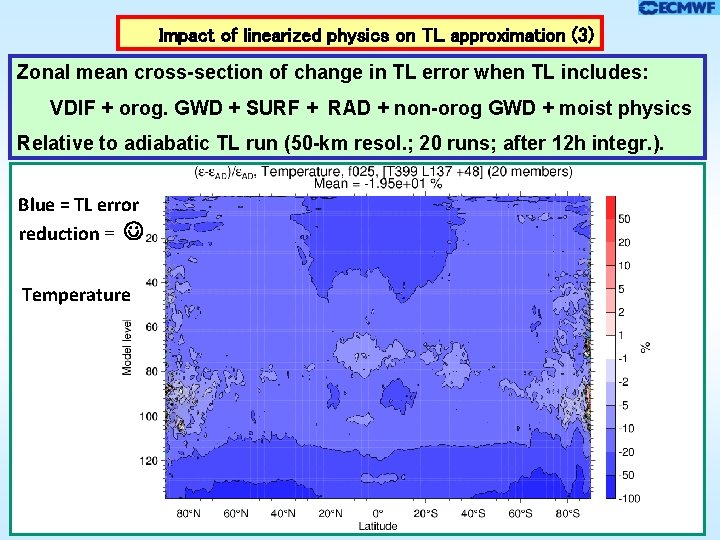
Impact of linearized physics on tangent-linear approximation Comparison: Finite difference of two NL integrations TL evolution of initial perturbations Examination of the accuracy of the linearization for typical analysis increments: typical size of 4 D-Var analysis increments Diagnostics: • mean absolute errors: • relative error change: • here: (improvement if < 0) REF = adiabatic run (i. e. no physical parametrizations in tangent-linear)

Impact of linearized physics on TL approximation (1) Zonal mean cross-section of change in TL error when TL includes: VDIF + orog. GWD + SURF Relative to adiabatic TL run (50 -km resol. ; 20 runs; after 12 h integr. ). Blue = TL error reduction = Temperature

Impact of linearized physics on TL approximation (2) Zonal mean cross-section of change in TL error when TL includes: VDIF + orog. GWD + SURF + RAD Relative to adiabatic TL run (50 -km resol. ; 20 runs; after 12 h integr. ). Blue = TL error reduction = Temperature

Impact of linearized physics on TL approximation (3) Zonal mean cross-section of change in TL error when TL includes: VDIF + orog. GWD + SURF + RAD + non-orog GWD + moist physics Relative to adiabatic TL run (50 -km resol. ; 20 runs; after 12 h integr. ). Blue = TL error reduction = Temperature

Applications

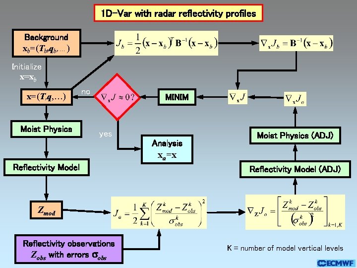
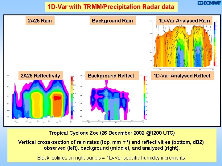
1 D-Var with radar reflectivity profiles Background xb=(Tb, qb, …) Initialize x=xb x=(T, q, …) Moist Physics no MINIM yes Analysis Moist Physics (ADJ) xa=x Reflectivity Model (ADJ) Zmod Reflectivity observations Zobs with errors obs K = number of model vertical levels

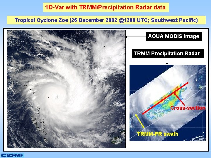
1 D-Var with TRMM/Precipitation Radar data Tropical Cyclone Zoe (26 December 2002 @1200 UTC; Southwest Pacific) AQUA MODIS image TRMM Precipitation Radar Cross-section TRMM-PR swath

1 D-Var with TRMM/Precipitation Radar data 2 A 25 Rain Background Rain 2 A 25 Reflectivity Background Reflect. 1 D-Var Analysed Rain 1 D-Var Analysed Reflect. Tropical Cyclone Zoe (26 December 2002 @1200 UTC) Vertical cross-section of rain rates (top, mm h-1) and reflectivities (bottom, d. BZ): observed (left), background (middle), and analyzed (right). Black isolines on right panels = 1 D-Var specific humidity increments.

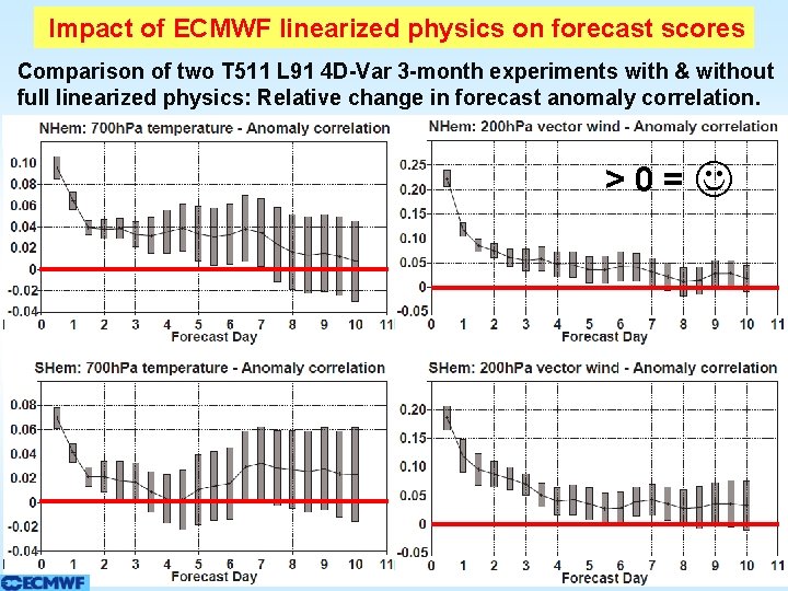
Impact of ECMWF linearized physics on forecast scores Comparison of two T 511 L 91 4 D-Var 3 -month experiments with & without full linearized physics: Relative change in forecast anomaly correlation. >0=

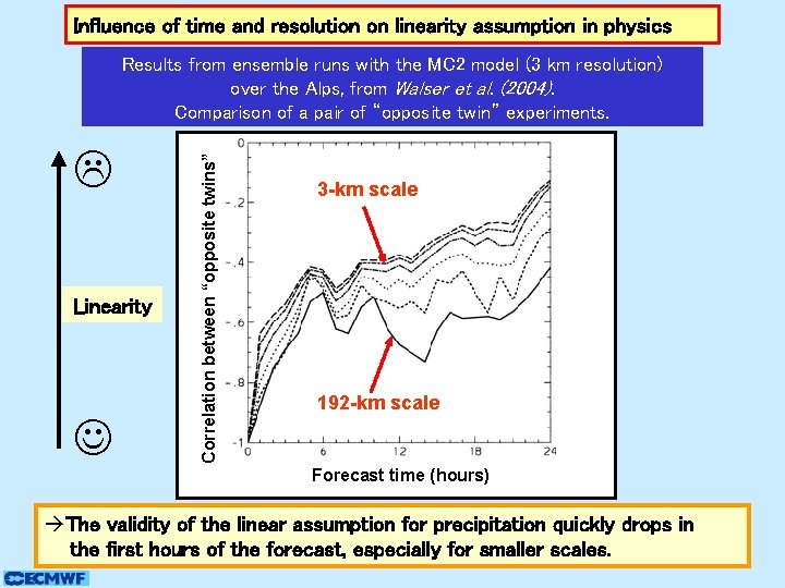
Influence of time and resolution on linearity assumption in physics Linearity Correlation between “opposite twins” Results from ensemble runs with the MC 2 model (3 km resolution) over the Alps, from Walser et al. (2004). Comparison of a pair of “opposite twin” experiments. 3 -km scale 192 -km scale Forecast time (hours) The validity of the linear assumption for precipitation quickly drops in the first hours of the forecast, especially for smaller scales.

Summary and prospects (1) • Linearized physical parameterizations have become essential components of variational data assimilation systems: Better representation of the evolution of the atmospheric state during the minimization of the cost function (via the adjoint model integration). Extraction of information from observations that are strongly affected by physical processes (e. g. by clouds or precipitation). · However, there are some limitations to the LP approach: 1) Theoretical: The domain of validity of the linear hypothesis shrinks with increasing resolution and integration length. 2) Technical: Linearized models require sustained & time-consuming attention: Testing tangent-linear approximation and adjoint code. Regularizations / simplifications to eliminate any source of instability. Revisions to ensure good match with reference non-linear forecast model.

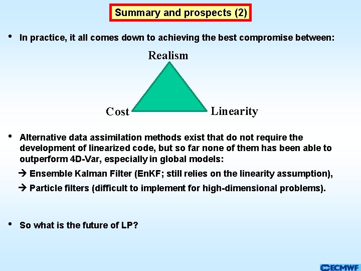
Summary and prospects (2) • In practice, it all comes down to achieving the best compromise between: Realism Cost • Linearity Alternative data assimilation methods exist that do not require the development of linearized code, but so far none of them has been able to outperform 4 D-Var, especially in global models: Ensemble Kalman Filter (En. KF; still relies on the linearity assumption), Particle filters (difficult to implement for high-dimensional problems). • So what is the future of LP?

Working on linearized physics may be tedious…

…but it is for the greater good.

Summary and prospects (3) • Eventually, it might become impractical or even impossible to make LP work efficiently at resolutions of a few kilometres, even if the linearity constraint can be relaxed (e. g. by using shorter 4 D-Var window or weak-constraint 4 DVar). ? Thank you!

Example of observation operator H (radiative transfer model): and its tangent-linear operator H:

REFERENCES • Variational data assimilation: Lorenc, A. , 1986, Quarterly Journal of the Royal Meteorological Society, 112, 1177 -1194. Courtier, P. et al. , 1994, Quarterly Journal of the Royal Meteorological Society, 120, 1367 -1387. Bouttier, F. and P. Courtier, 1999: Data assimilation concepts and methods, ECMWF lecture notes, available at http: //www. ecmwf. int/newsevents/training/lecture_notes/LN_DA. html. Rabier, F. et al. , 2000, Quarterly Journal of the Royal Meteorological Society, 126, 1143 -1170. • The adjoint technique: Errico, R. M. , 1997, Bulletin of the American Meteorological Society, 78, 2577 -2591. • Tangent-linear approximation: Errico, R. M. et al. , 1993, Tellus, 45 A, 462 -477. Errico, R. M. , and K. Reader, 1999, Quarterly Journal of the Royal Meteorological Society, 125, 169 -195. Janisková, M. et al. , 1999, Monthly Weather Review, 127, 26 -45. . • Physical parameterizations for data assimilation: Mahfouf, J. -F. , 1999, Tellus, 51 A, 147 -166. Janisková, M. et al. , 2002, Quarterly Journal of the Royal Meteorological Society, 128, 1505 -1527. Tompkins, A. M. , and M. Janisková, 2004, Quarterly Journal of the Royal Meteorological Society, 130, 2495 -2518. Lopez, P. , and E. Moreau, 2005, Quarterly Journal of the Royal Meteorological Society, 131, 409 -436. Janisková, M. , and P. Lopez, 2012: Linearized physics for data assimilation at ECMWF, Technical Memorandum 666, available from ECMWF, Reading, UK.

REFERENCES • Microwave Radiative Transfer Model for data assimilation: Bauer, P. , May 2002, Satellite Application Facility for Numerical Weather Prediction NWPSAF-ECTR-005, 27 pages. • Assimilation of observations affected by precipitation and/or clouds: Lopez, P. 2007: Journal Atmospheric Sciences, Special Issue on the Assimilation of Satellite Cloud and Precipitation Observations in NWP Models, 64, 3770 -3788 (Review paper on the use of moist physical parameterizations in data assimilation). Bauer, P. Lopez, A. Benedetti, D. Salmond, and E. Moreau, 2006 a, Quarterly Journal of the Royal Meteorological Society, 132, 2277 -2306. Bauer, P. Lopez, A. Benedetti, D. Salmond, S. Saarinen, and M. Bonazzola, 2006 b, Quarterly Journal of the Royal Meteorological Society, 132, 2307 -2332. Fillion, L. , and R. M. Errico, 1997, Monthly Weather Review, 125, 2917 -2942. Ducrocq, V. , et al. , 2000, Quarterly Journal of the Royal Meteorological Society, 126, 3041 -3065. Hou, A. et al. , 2000, Monthly Weather Review, 128, 509 -537. Marécal, V. , and. J. -F. Mahfouf, 2002, Monthly Weather Review, 130, 43 -58. Marécal, V. , and. J. -F. Mahfouf, 2003, Quarterly Journal of the Royal Meteorological Society, 129, 3137 -3160.