OnShell Methods in Quantum Field Theory David A

On-Shell Methods in Quantum Field Theory David A. Kosower Institut de Physique Théorique, CEA–Saclay LHC Pheno. Net Summer School Cracow, Poland September 7– 12, 2013

Tools for Computing Amplitudes • New tools for computing in gauge theories — the core of the Standard Model • Motivations and connections – Particle physics: SU(3) SU(2) U(1) – N = 4 supersymmetric gauge theories and Ad. S/CFT – Witten’s twistor string – Grassmanians – N = 8 supergravity

• The particle content of the Standard Model is now complete, with last year’s discovery of a Higgs-like boson by the ATLAS and CMS collaborations • Every discovery opens new doors, and raises new questions • How Standard-Model-like is the new boson? – We’ll need precision calculations to see • Is there anything else hiding in the LHC data? – We’ll need background calculations to know

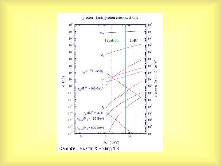
Campbell, Huston & Stirling ‘ 06

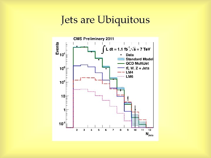
Jets are Ubiquitous

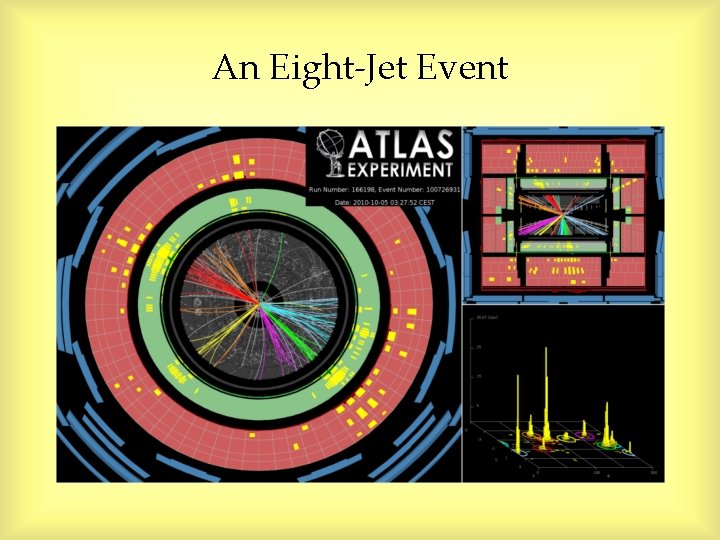
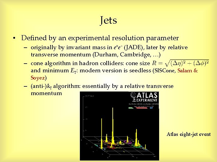
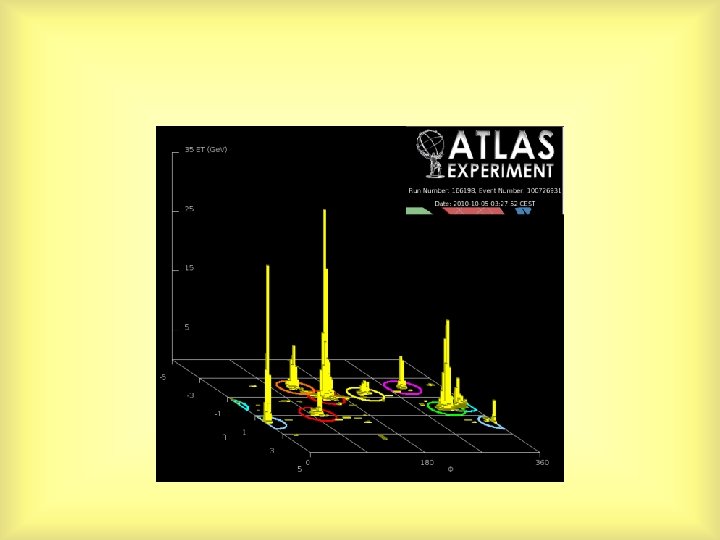
An Eight-Jet Event

Jets are Ubiquitous

• Complexity is due to QCD • Perturbative QCD: Gluons & quarks → gluons & quarks • Real world: Hadrons → hadrons with hard physics described by p. QCD • Hadrons → jets narrow nearly collimated streams of hadrons

Jets • Defined by an experimental resolution parameter – originally by invariant mass in e+e− (JADE), later by relative transverse momentum (Durham, Cambridge, …) – cone algorithm in hadron colliders: cone size and minimum ET: modern version is seedless (SISCone, Salam & Soyez) – (anti-)k. T algorithm: essentially by a relative transverse momentum Atlas eight-jet event

In theory, theory and practice are the same. In practice, they are different — Yogi Berra

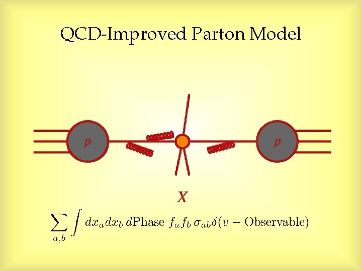
QCD-Improved Parton Model

The Challenge • Everything at a hadron collider (signals, backgrounds, luminosity measurement) involves QCD • Strong coupling is not small: s(MZ) 0. 12 and running is important events have high multiplicity of hard clusters (jets) each jet has a high multiplicity of hadrons higher-order perturbative corrections are important • Processes can involve multiple scales: p. T(W) & MW need resummation of logarithms • Confinement introduces further issues of mapping partons to hadrons, but for suitably-averaged quantities (infrared-safe) avoiding small E scales, this is not a problem (power corrections)

Approaches • General parton-level fixed-order calculations – Numerical jet programs: general observables – Systematic to higher order/high multiplicity in perturbation theory – Parton-level, approximate jet algorithm; match detector events only statistically • Parton showers Peter Skands’s lectures – General observables – Leading- or next-to-leading logs only, approximate for higher order/high multiplicity – Can hadronize & look at detector response event-by-event – Understood how to match to matrix elements at leading order • Semi-analytic calculations/resummations – Specific observable, for high-value targets – Checks on general fixed-order calculations

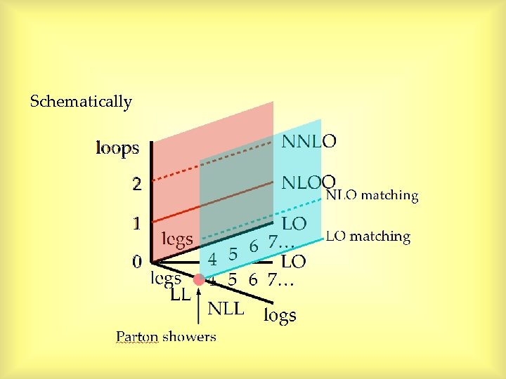
Schematically

Precision Perturbative QCD • • • Predictions of signals, signals+jets Predictions of backgrounds Everything at a hadron Measurement of luminosity collider involves QCD Measurement of fundamental parameters ( s, mt) Measurement of electroweak parameters Extraction of parton distributions — ingredients in any theoretical prediction

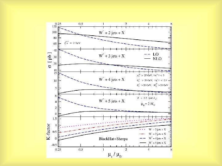
Renormalization Scale • Needed to define the coupling • Physical quantities should be independent of it • Truncated perturbation theory isn’t • Dependence is ~ the first missing order * logs • Similarly for factorization scale — define parton distributions

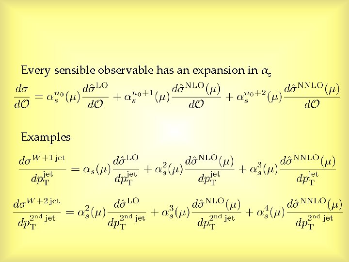
Every sensible observable has an expansion in αs Examples

Leading-Order, Next-to-Leading Order • QCD at LO is not quantitative • LO: Basic shapes of distributions but: no quantitative prediction — large dependence on unphysical renormalization and factorization scales missing sensitivity to jet structure & energy flow • NLO: First quantitative prediction, expect it to be reliable to 10– 15% improved scale dependence — inclusion of virtual corrections basic approximation to jet structure — jet = 2 partons importance grows with increasing number of jets • NNLO: Precision predictions small scale dependence better correspondence to experimental jet algorithms understanding of theoretical uncertainties will be required for <5% predictions for future precision measurements

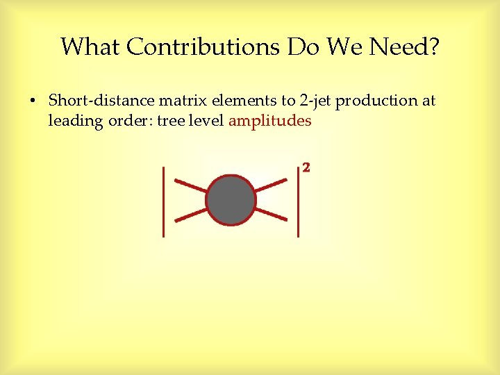
What Contributions Do We Need? • Short-distance matrix elements to 2 -jet production at leading order: tree level amplitudes

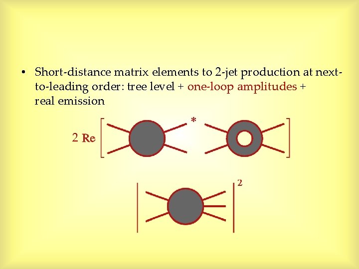
• Short-distance matrix elements to 2 -jet production at nextto-leading order: tree level + one-loop amplitudes + real emission 2

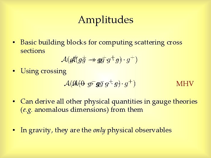
Amplitudes • Basic building blocks for computing scattering cross sections • Using crossing MHV • Can derive all other physical quantities in gauge theories (e. g. anomalous dimensions) from them • In gravity, they are the only physical observables

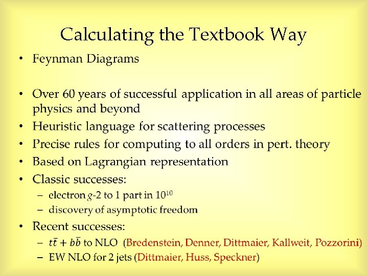
Calculating the Textbook Way •

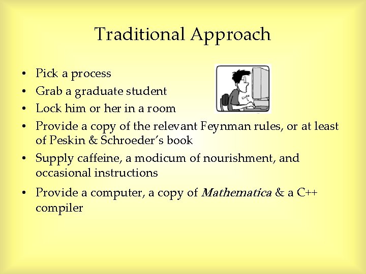
Traditional Approach Pick a process Grab a graduate student Lock him or her in a room Provide a copy of the relevant Feynman rules, or at least of Peskin & Schroeder’s book • Supply caffeine, a modicum of nourishment, and occasional instructions • • • Provide a computer, a copy of Mathematica & a C++ compiler

A Difficulty • Huge number of diagrams in calculations of interest — factorial growth • 2 → 6 jets: 34300 tree diagrams, ~ 2. 5 ∙ 107 terms ~2. 9 ∙ 106 1 -loop diagrams, ~ 1. 9 ∙ 1010 terms

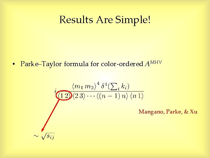
Results Are Simple! • Parke–Taylor formula for color-ordered AMHV Mangano, Parke, & Xu

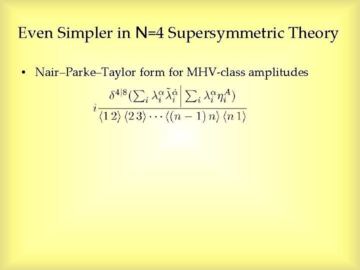
Even Simpler in N=4 Supersymmetric Theory • Nair–Parke–Taylor form for MHV-class amplitudes

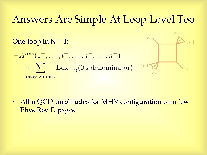
Answers Are Simple At Loop Level Too One-loop in N = 4: • All-n QCD amplitudes for MHV configuration on a few Phys Rev D pages

Calculation is a Mess • Vertices and propagators involve gauge-variant off-shell states • Each diagram is not gauge-invariant — huge cancellations of gauge-noninvariant, redundant, parts are to blame (exacerbated by high-rank tensor reductions)

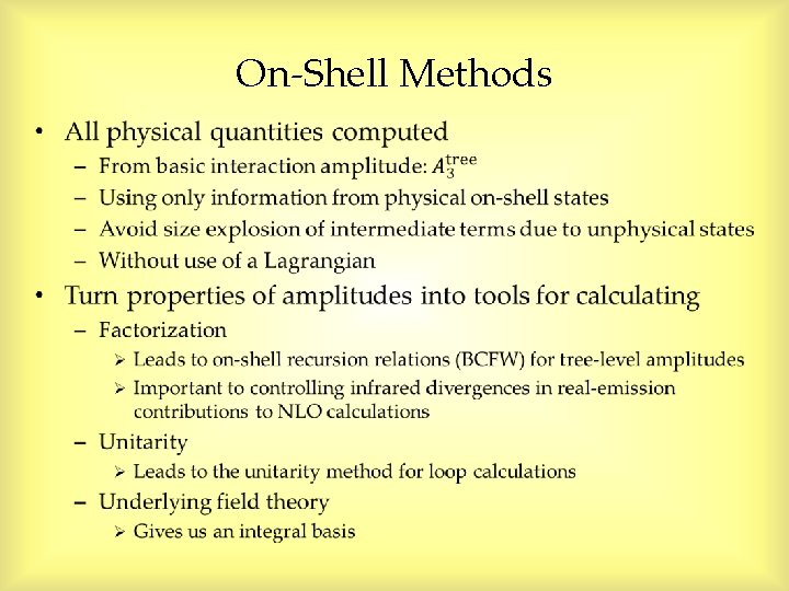
On-Shell Methods •

On-Shell Methods • Kinematics: spinor variables • Properties of amplitudes become calculational tools Ø Factorization → on-shell recursion (Britto, Cachazo, Feng, Witten, …) Ø Unitarity → unitarity method (Bern, Dixon, Dunbar, DAK, …) Ø Underlying field theory → integral basis

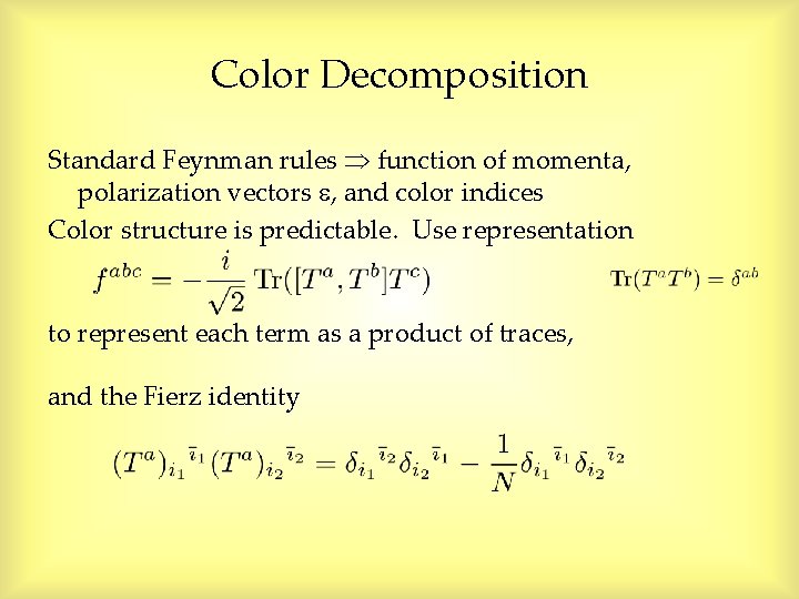
Color Decomposition Standard Feynman rules function of momenta, polarization vectors , and color indices Color structure is predictable. Use representation to represent each term as a product of traces, and the Fierz identity

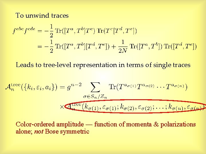
To unwind traces Leads to tree-level representation in terms of single traces Color-ordered amplitude — function of momenta & polarizations alone; not Bose symmetric

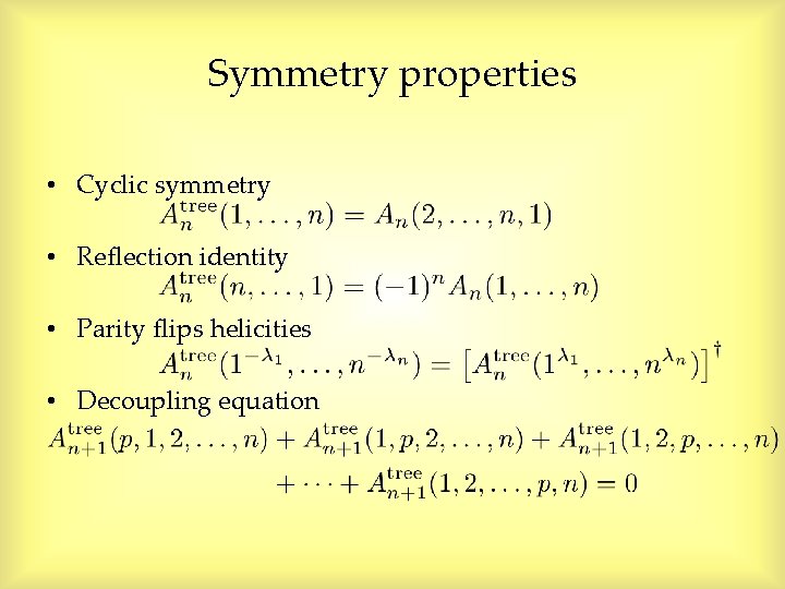
Symmetry properties • Cyclic symmetry • Reflection identity • Parity flips helicities • Decoupling equation

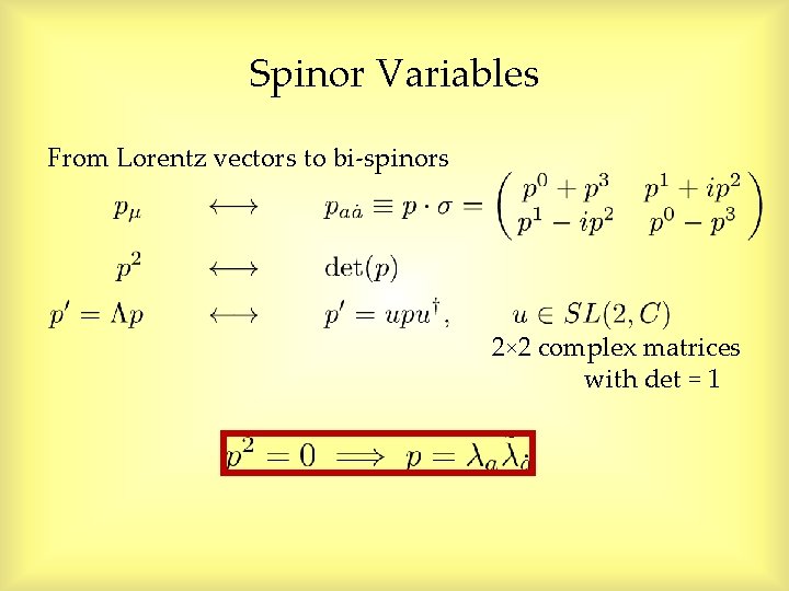
Spinor Variables From Lorentz vectors to bi-spinors 2× 2 complex matrices with det = 1

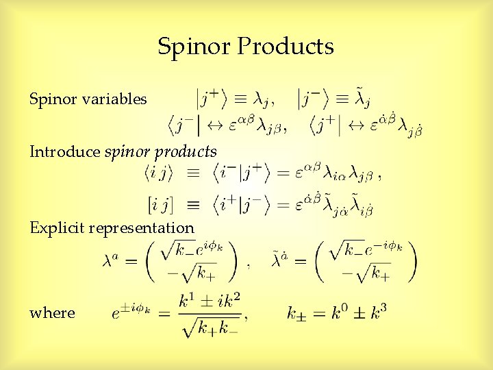
Spinor Products Spinor variables Introduce spinor products Explicit representation where

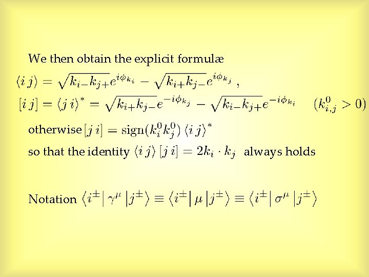
We then obtain the explicit formulæ otherwise so that the identity always holds Notation

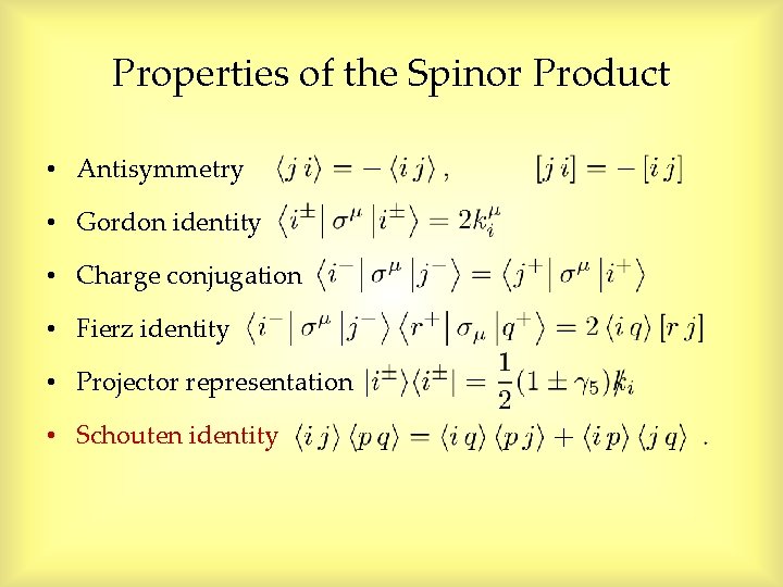
Properties of the Spinor Product • Antisymmetry • Gordon identity • Charge conjugation • Fierz identity • Projector representation • Schouten identity

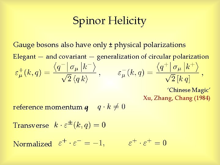
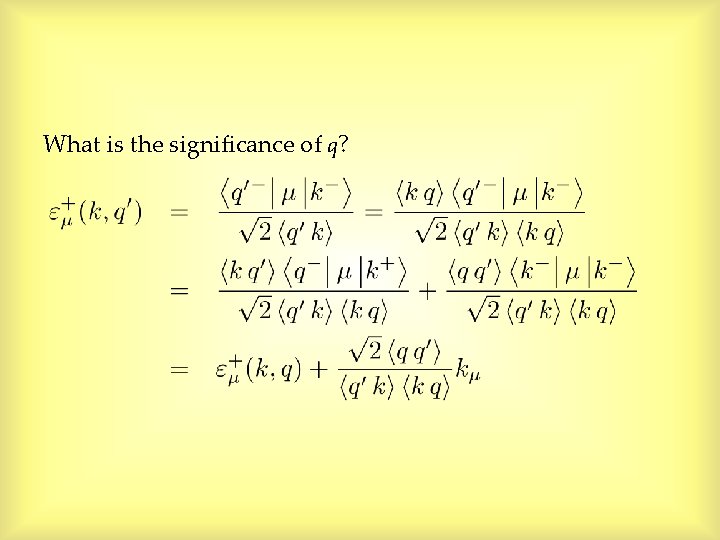
Spinor Helicity Gauge bosons also have only ± physical polarizations Elegant — and covariant — generalization of circular polarization reference momentum q Transverse Normalized ‘Chinese Magic’ Xu, Zhang, Chang (1984)

What is the significance of q?

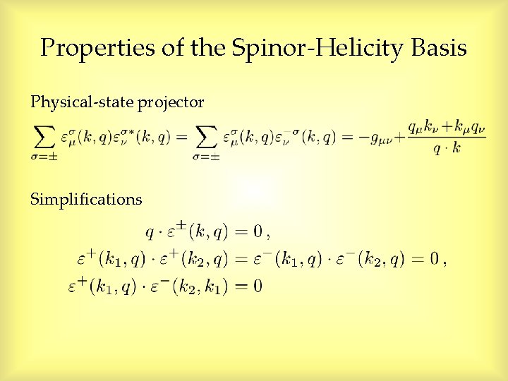
Properties of the Spinor-Helicity Basis Physical-state projector Simplifications

A Mathematica Implementation: S@M Maitre and Mastrolia (0710. 5559)

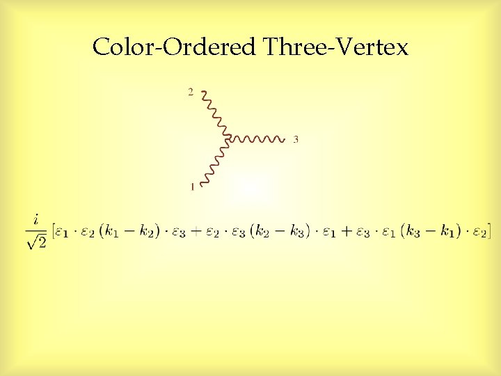
Color-Ordered Three-Vertex

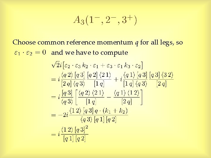
Choose common reference momentum q for all legs, so and we have to compute

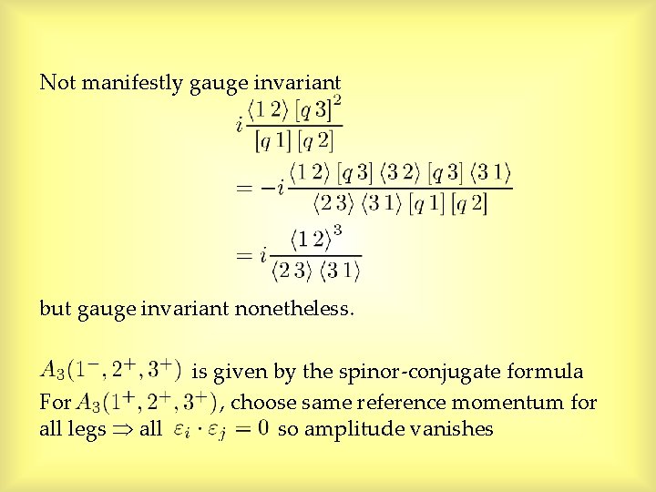
Not manifestly gauge invariant but gauge invariant nonetheless. is given by the spinor-conjugate formula For , choose same reference momentum for all legs all so amplitude vanishes

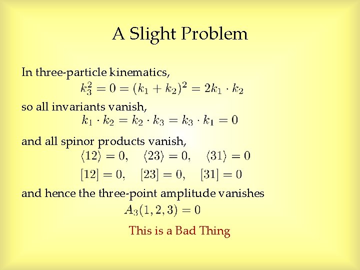
A Slight Problem In three-particle kinematics, so all invariants vanish, and all spinor products vanish, and hence three-point amplitude vanishes This is a Bad Thing

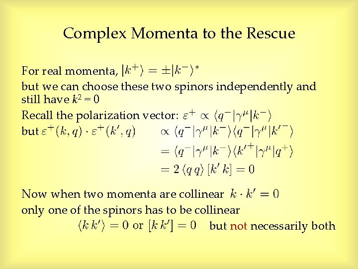
Complex Momenta to the Rescue For real momenta, but we can choose these two spinors independently and still have k 2 = 0 Recall the polarization vector: but Now when two momenta are collinear only one of the spinors has to be collinear but not necessarily both