Nonparametrics and goodnessoffit Tron Anders Moger 23 10

Nonparametrics and goodness-offit Tron Anders Moger 23. 10. 2006

Nonparametric statistics • In tests we have done so far, the null hypothesis has always been a stochastic model with a few parameters. – – T tests Tests for regression coefficients Test for autocorrelation … • In nonparametric tests, the null hypothesis is not a parametric distribution, rather a much larger class of possible distributions

Parametric methods we’ve seen: • Estimation – Confidence interval for µ 1 -µ 2 • Testing – One sample T test – Two sample T test • The methods are based on the assumption of normally distributed data (or normally distributed mean)

Nonparametric statistics • The null hypothesis is for example that the median of the distribution is zero • A test statistic can be formulated, so that – it has a known distribution under this hypothesis – it has more extreme values under alternative hypotheses

Non-parametric methods: • Estimation – Confidence interval for the median • Testing – Paired data: Sign test and Wilcoxon signed rank test – Two independent samples: Mann-Whitney test/Wilcoxon rank-sum test • Make (almost) no assumptions regarding distribution

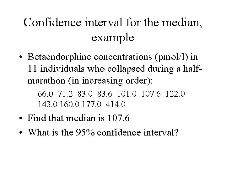
Confidence interval for the median, example • Betaendorphine concentrations (pmol/l) in 11 individuals who collapsed during a halfmarathon (in increasing order): 66. 0 71. 2 83. 0 83. 6 101. 0 107. 6 122. 0 143. 0 160. 0 177. 0 414. 0 • Find that median is 107. 6 • What is the 95% confidence interval?

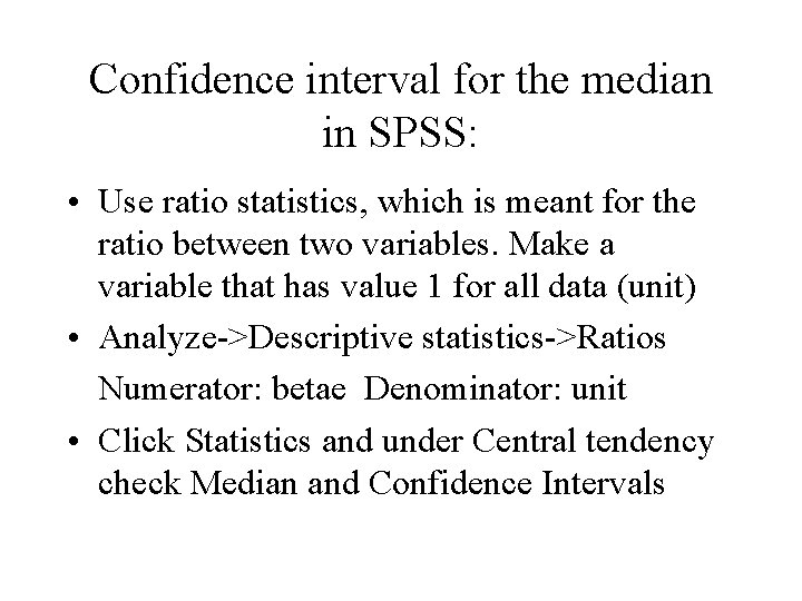
Confidence interval for the median in SPSS: • Use ratio statistics, which is meant for the ratio between two variables. Make a variable that has value 1 for all data (unit) • Analyze->Descriptive statistics->Ratios Numerator: betae Denominator: unit • Click Statistics and under Central tendency check Median and Confidence Intervals

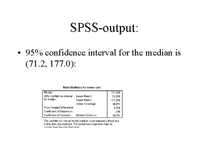
SPSS-output: • 95% confidence interval for the median is (71. 2, 177. 0):

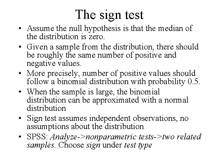
The sign test • Assume the null hypothesis is that the median of the distribution is zero. • Given a sample from the distribution, there should be roughly the same number of positive and negative values. • More precisely, number of positive values should follow a binomial distribution with probability 0. 5. • When the sample is large, the binomial distribution can be approximated with a normal distribution • Sign test assumes independent observations, no assumptions about the distribution • SPSS: Analyze->nonparametric tests->two related samples. Choose sign under test type

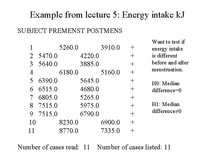
Example from lecture 5: Energy intake k. J SUBJECT PREMENST POSTMENS 1 2 3 4 5 6 7 8 9 10 11 5260. 0 5470. 0 5640. 0 3910. 0 4220. 0 3885. 0 6180. 0 6390. 0 6515. 0 6805. 0 7515. 0 5160. 0 5645. 0 4680. 0 5265. 0 5975. 0 6790. 0 8230. 0 8770. 0 Number of cases read: 11 6900. 0 7335. 0 + + + Want to test if energy intake is different before and after menstruation. H 0: Median difference=0 H 1: Median difference≠ 0 Number of cases listed: 11

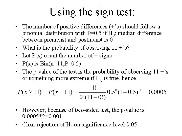
Using the sign test: • The number of positive differences (+’s) should follow a binomial distribution with P=0. 5 if H 0: median difference between premenst and postmenst is 0 • What is the probability of observing 11 +’s? • Let P(x) count the number of + signs • P(x) is Bin(n=11, P=0. 5) • The p-value of the test is the probability of observing 11 +’s or something more extreme if H 0 is true, hence • However, because of two-sided test, the p-value is 0. 0005*2=0. 001 • Clear rejection of H 0 on significance-level 0. 05

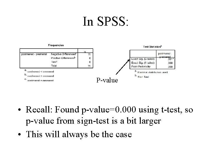
In SPSS: P-value • Recall: Found p-value=0. 000 using t-test, so p-value from sign-test is a bit larger • This will always be the case

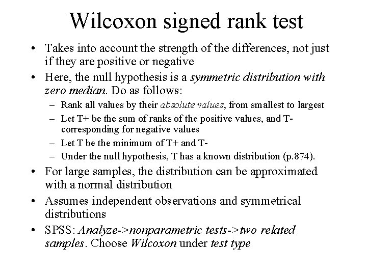
Wilcoxon signed rank test • Takes into account the strength of the differences, not just if they are positive or negative • Here, the null hypothesis is a symmetric distribution with zero median. Do as follows: – Rank all values by their absolute values, from smallest to largest – Let T+ be the sum of ranks of the positive values, and Tcorresponding for negative values – Let T be the minimum of T+ and T– Under the null hypothesis, T has a known distribution (p. 874). • For large samples, the distribution can be approximated with a normal distribution • Assumes independent observations and symmetrical distributions • SPSS: Analyze->nonparametric tests->two related samples. Choose Wilcoxon under test type

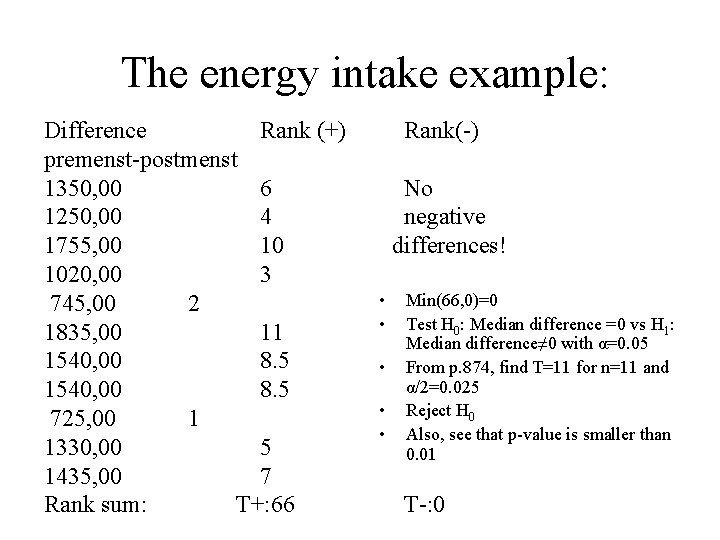
The energy intake example: Difference Rank (+) premenst-postmenst 1350, 00 6 1250, 00 4 1755, 00 10 1020, 00 3 745, 00 2 1835, 00 11 1540, 00 8. 5 725, 00 1 1330, 00 5 1435, 00 7 Rank sum: T+: 66 Rank(-) No negative differences! • • • Min(66, 0)=0 Test H 0: Median difference =0 vs H 1: Median difference≠ 0 with α=0. 05 From p. 874, find T=11 for n=11 and α/2=0. 025 Reject H 0 Also, see that p-value is smaller than 0. 01 T-: 0

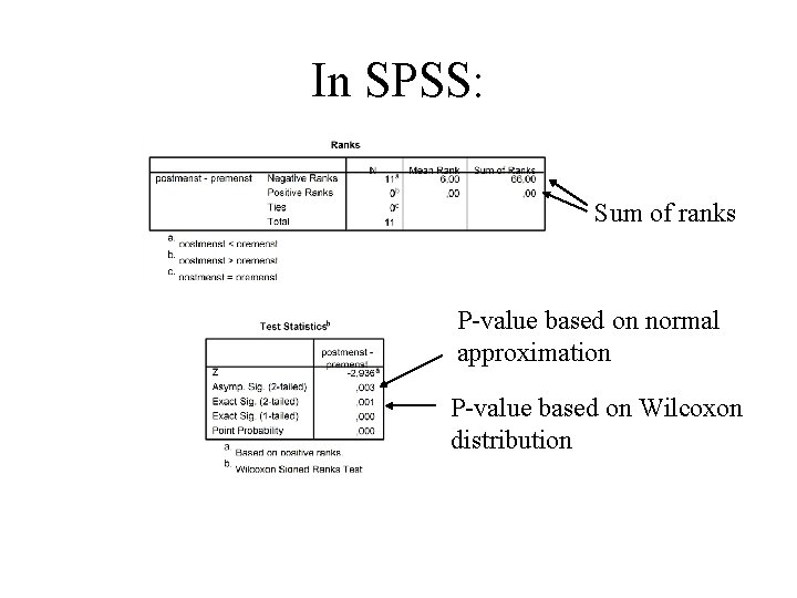
In SPSS: Sum of ranks P-value based on normal approximation P-value based on Wilcoxon distribution

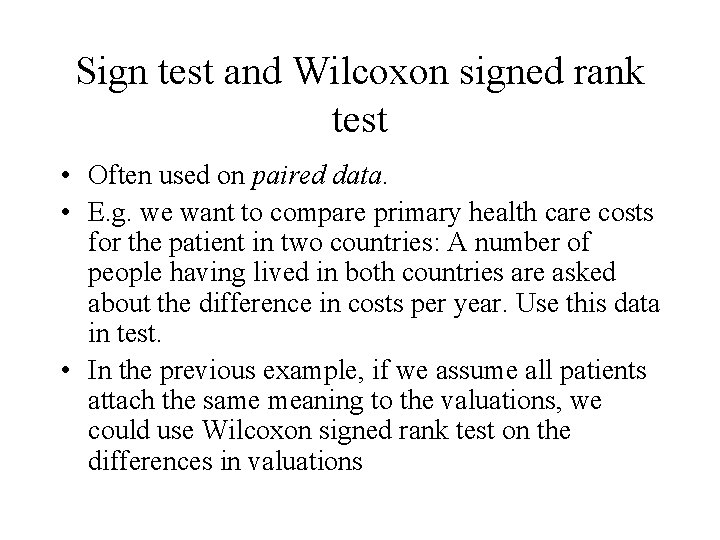
Sign test and Wilcoxon signed rank test • Often used on paired data. • E. g. we want to compare primary health care costs for the patient in two countries: A number of people having lived in both countries are asked about the difference in costs per year. Use this data in test. • In the previous example, if we assume all patients attach the same meaning to the valuations, we could use Wilcoxon signed rank test on the differences in valuations

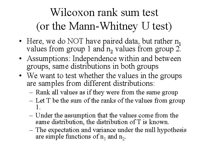
Wilcoxon rank sum test (or the Mann-Whitney U test) • Here, we do NOT have paired data, but rather n 1 values from group 1 and n 2 values from group 2. • Assumptions: Independence within and between groups, same distributions in both groups • We want to test whether the values in the groups are samples from different distributions: – Rank all values as if they were from the same group – Let T be the sum of the ranks of the values from group 1. – Under the assumption that the values come from the same distribution, the distribution of T is known. – The expectation and variance under the null hypothesis are simple functions of n 1 and n 2.

Wilcoxon rank sum test (or the Mann-Whitney U test) • For large samples, we can use a normal approximation for the distribution of T. • The Mann-Whitney U test gives exactly the same results, but uses slightly different test statistic. • In SPSS: – Analyze->nonparametric tests-> two independent samples tests – Test type: Mann-Whitney U

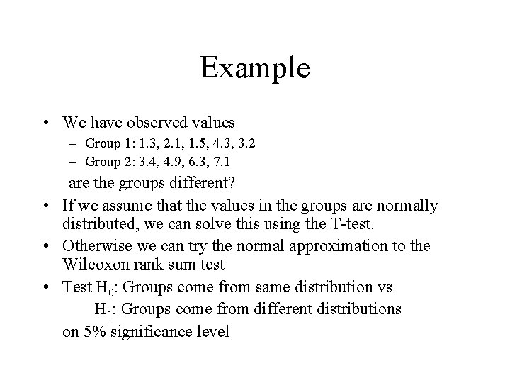
Example • We have observed values – Group 1: 1. 3, 2. 1, 1. 5, 4. 3, 3. 2 – Group 2: 3. 4, 4. 9, 6. 3, 7. 1 are the groups different? • If we assume that the values in the groups are normally distributed, we can solve this using the T-test. • Otherwise we can try the normal approximation to the Wilcoxon rank sum test • Test H 0: Groups come from same distribution vs H 1: Groups come from different distributions on 5% significance level

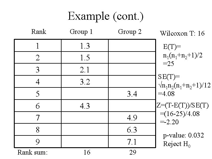
Example (cont. ) Rank 1 2 3 4 5 6 7 8 9 Rank sum: Group 1 Group 2 1. 3 1. 5 2. 1 3. 2 E(T)= n 1(n 1+n 2+1)/2 =25 3. 4 4. 3 4. 9 6. 3 7. 1 16 Wilcoxon T: 16 29 SE(T)= √n 1 n 2(n 1+n 2+1)/12 =4. 08 Z=(T-E(T))/SE(T) =(16 -25)/4. 08 =-2. 20 p-value: 0. 032 Reject H 0

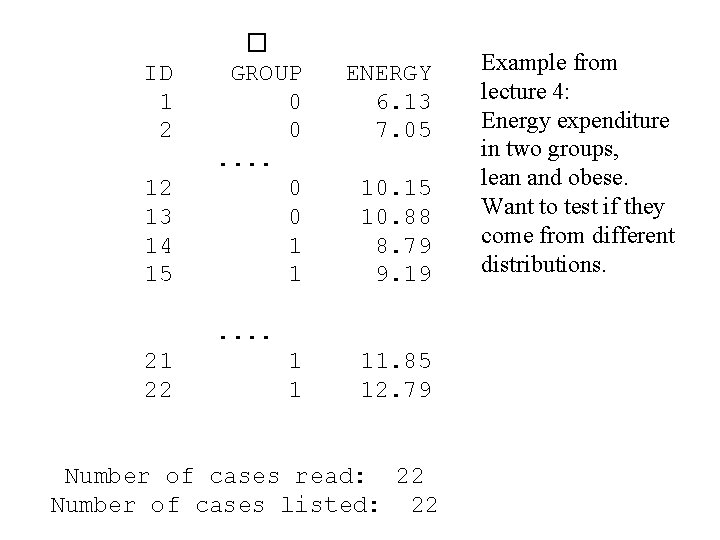
ID 1 2 12 13 14 15 � GROUP 0 0. . 0 0 1 1 ENERGY 6. 13 7. 05 10. 15 10. 88 8. 79 9. 19 . . 21 22 1 1 11. 85 12. 79 Number of cases read: 22 Number of cases listed: 22 Example from lecture 4: Energy expenditure in two groups, lean and obese. Want to test if they come from different distributions.

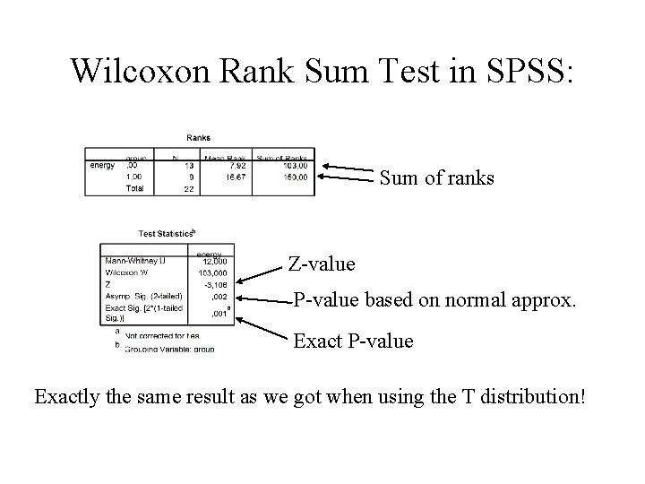
Wilcoxon Rank Sum Test in SPSS: Sum of ranks Z-value P-value based on normal approx. Exact P-value Exactly the same result as we got when using the T distribution!

Spearman rank correlation • This can be applied when you have two observations per item, and you want to test whether the observations are related. • Computing the sample correlation (Pearson’s r) gives an indication. • We can test whether the Pearson correlation could be zero but test needs assumption of normality.

Spearman rank correlation • The Spearman rank correlation tests for association without any assumption on the association: – Rank the X-values, and rank the Y-values. – Compute ordinary sample correlation of the ranks: This is called the Spearman rank correlation. – Under the null hypothesis that X values and Y values are independent, it has a fixed, tabulated distribution (depending on number of observations)

Concluding remarks on nonparametric statistics • Tests with much more general null hypotheses, and so fewer assumptions • Often a good choice when normality of the data cannot be assumed • If you reject the null hypothesis with a nonparametric test, it is a robust conclusion • However, with small amounts of data, you can often not get significant conclusions • In SPSS, you only get p-values from nonparametric tests, more interesting to know the mean difference and confidence intervals

Some useful comments: • Always start by checking whether it is appropriate to use T tests (normally distributed data) • If in doubt, a useful tip is to compare pvalues from t-tests with p-values from nonparametric tests • If very different results, stay with the pvalues from the non-parametric tests

Contingency tables • The following data type is frequent: Each object (person, case, …) can be in one of two or more categories. The data is the count of number of objects in each category. • Often, you measure several categories for each object. The resulting counts can then be put in a contingency table.

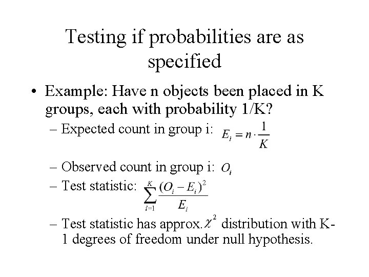
Testing if probabilities are as specified • Example: Have n objects been placed in K groups, each with probability 1/K? – Expected count in group i: – Observed count in group i: – Test statistic has approx. distribution with K 1 degrees of freedom under null hypothesis.

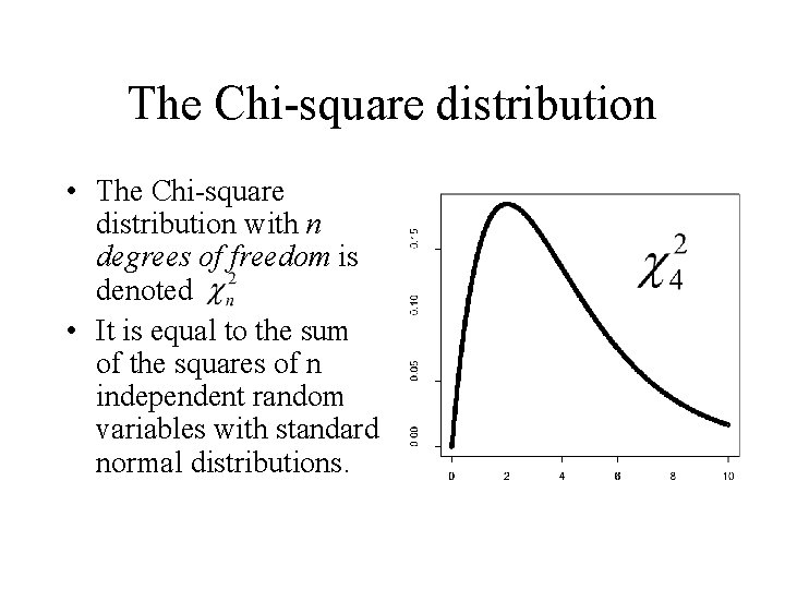
The Chi-square distribution • The Chi-square distribution with n degrees of freedom is denoted • It is equal to the sum of the squares of n independent random variables with standard normal distributions.

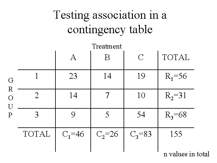
Testing association in a contingency table Treatment G R O U P A B C TOTAL 1 23 14 19 R 1=56 2 14 7 10 R 2=31 3 9 5 54 R 3=68 TOTAL C 1=46 C 2=26 C 3=83 155 n values in total

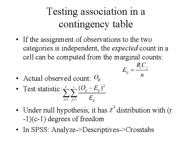
Testing association in a contingency table • If the assignment of observations to the two categories is independent, the expected count in a cell can be computed from the marginal counts: • Actual observed count: • Test statistic: • Under null hypothesis, it has distribution with (r -1)(c-1) degrees of freedom • In SPSS: Analyze->Descriptives->Crosstabs

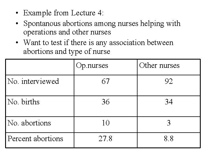
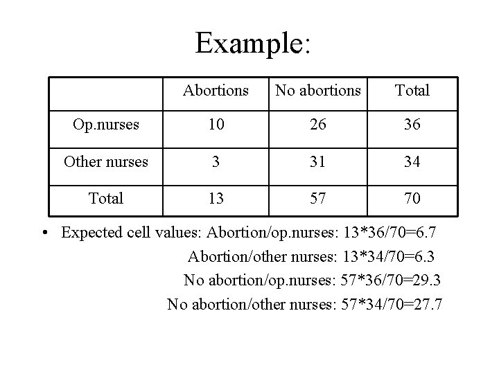
• Example from Lecture 4: • Spontanous abortions among nurses helping with operations and other nurses • Want to test if there is any association between abortions and type of nurse Op. nurses Other nurses No. interviewed 67 92 No. births 36 34 No. abortions 10 3 27. 8 8. 8 Percent abortions

Example: Abortions No abortions Total Op. nurses 10 26 36 Other nurses 3 31 34 Total 13 57 70 • Expected cell values: Abortion/op. nurses: 13*36/70=6. 7 Abortion/other nurses: 13*34/70=6. 3 No abortion/op. nurses: 57*36/70=29. 3 No abortion/other nurses: 57*34/70=27. 7

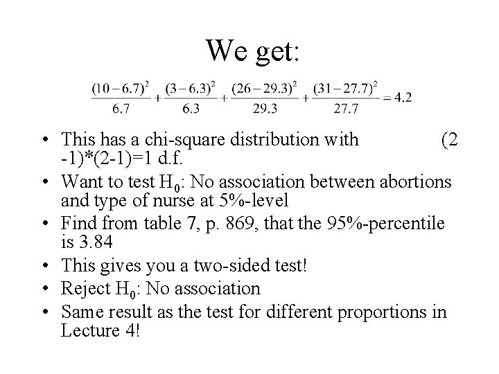
We get: • This has a chi-square distribution with (2 -1)*(2 -1)=1 d. f. • Want to test H 0: No association between abortions and type of nurse at 5%-level • Find from table 7, p. 869, that the 95%-percentile is 3. 84 • This gives you a two-sided test! • Reject H 0: No association • Same result as the test for different proportions in Lecture 4!

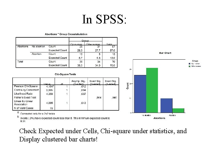
In SPSS: Check Expected under Cells, Chi-square under statistics, and Display clustered bar charts!

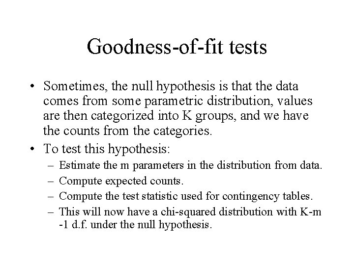
Goodness-of-fit tests • Sometimes, the null hypothesis is that the data comes from some parametric distribution, values are then categorized into K groups, and we have the counts from the categories. • To test this hypothesis: – – Estimate the m parameters in the distribution from data. Compute expected counts. Compute the test statistic used for contingency tables. This will now have a chi-squared distribution with K-m -1 d. f. under the null hypothesis.

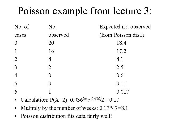
Poisson example from lecture 3: No. of No. Expected no. observed cases observed (from Poisson dist. ) 0 20 18. 4 1 16 17. 2 2 8 8. 1 3 2 2. 5 4 0 0. 6 5 0 0. 11 6 1 0. 017 • Calculation: P(X=2)=0. 9362*e-0. 936/2!=0. 17 • Multiply by the number of weeks: 0. 17*47=8. 1 • Poisson distribution fits data fairly well!

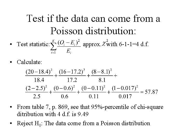
Test if the data can come from a Poisson distribution: • Test statistic: approx. with 6 -1 -1=4 d. f. • Calculate: • From table 7, p. 869, see that 95%-percentile of chi-square ditribution with 4 d. f. is 9. 49 • Reject H 0: The data come from a Poisson distribution

Tests for normality • Visual methods, like histograms and normality plots, are very useful. • In addition, several statistical tests for normality exist: – Kolmogorov-Smirnov test (which I have showed you before) – Bowman-Shelton test (tests skewness and kurtosis) • However, with enough data, visual methods are more useful

Next time: • Seen tests for comparing means in two independent groups • What if you have more than two groups? • Analysis of variance