Niedokoczone tematy Wodzisaw Duch Department of Informatics Nicolaus

Niedokończone tematy Włodzisław Duch Department of Informatics, Nicolaus Copernicus University, Toruń, Poland Google: W. Duch KIS, 25/04/2016

Projekty na inne tematy Neurocognitive Informatics: understanding complex cognition => creating algorithms that work in similar way. • • • Computational creativity, insight, intuition, imagery. Imagery agnosia, amusia, musical talent. Neurocognitive approach to language, word games. Brain stem models & consciousness in artificial systems. Medical information retrieval, analysis, visualization. Comprehensive theory of autism, ADHD, phenomics, education. Understanding neurodynamics, EEG signals, neurofeedback. Geometric theory of brain-mind processes. Infants: observation, guided development. Neural determinism, free will & social consequences.

Projekty CI Google Duch W => List of projects, talks, papers Computational intelligence (CI), main themes: • Understanding of data: visualization, prototype-based rules. • Foundations of computational intelligence: transformation based learning, k-separability, learning hard boole’an problems. • Novel learning: projection pursuit networks, QPC (Quality of Projected Clusters), search-based neural training, transfer learning or learning from others (ULM), a. RPM, SFM. . . • Similarity based framework for metalearning, heterogeneous systems, new transfer functions for neural networks. • Feature selection, extraction, creation of enhanced spaces. • General meta-learning, or learning how to learn, deep learning.

NN - wizualizacja 28. Visualization of the hidden node activity, or hidden secrets of neural networks. (PPT, 2. 2 MB), ICAISC Zakopane, Poland, June 2004 1. Wizualizacja funkcji NN w przestrzeni – dane + szum dają obraz w p-nie wyjściowej, ocena wiarygodności mapowania, zbieżności, wpływu regularyzacji, typu sieci itp. (WD). • • Duch W, Internal representations of multi-layered perceptrons. Issues in Intelligent Systems: Paradigms. 2005, pp. 49 -62. • Duch W, Visualization of hidden node activity in neural networks: I. Visualization methods. ICAISC 2004, LN in AI Vol. 3070 (2004) 38 -43; 44 -49 Cyt. 32 Więcej: http: //www. is. umk. pl/projects/nnv. html

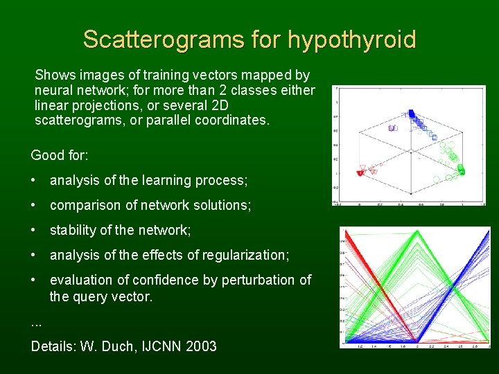
Scatterograms for hypothyroid Shows images of training vectors mapped by neural network; for more than 2 classes either linear projections, or several 2 D scatterograms, or parallel coordinates. Good for: • analysis of the learning process; • comparison of network solutions; • stability of the network; • analysis of the effects of regularization; • evaluation of confidence by perturbation of the query vector. . Details: W. Duch, IJCNN 2003

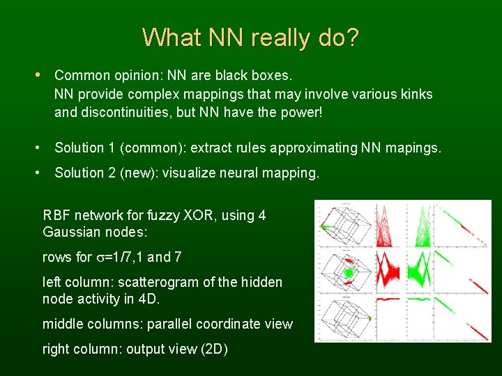
What NN really do? • Common opinion: NN are black boxes. NN provide complex mappings that may involve various kinks and discontinuities, but NN have the power! • Solution 1 (common): extract rules approximating NN mapings. • Solution 2 (new): visualize neural mapping. RBF network for fuzzy XOR, using 4 Gaussian nodes: rows for s=1/7, 1 and 7 left column: scatterogram of the hidden node activity in 4 D. middle columns: parallel coordinate view right column: output view (2 D)

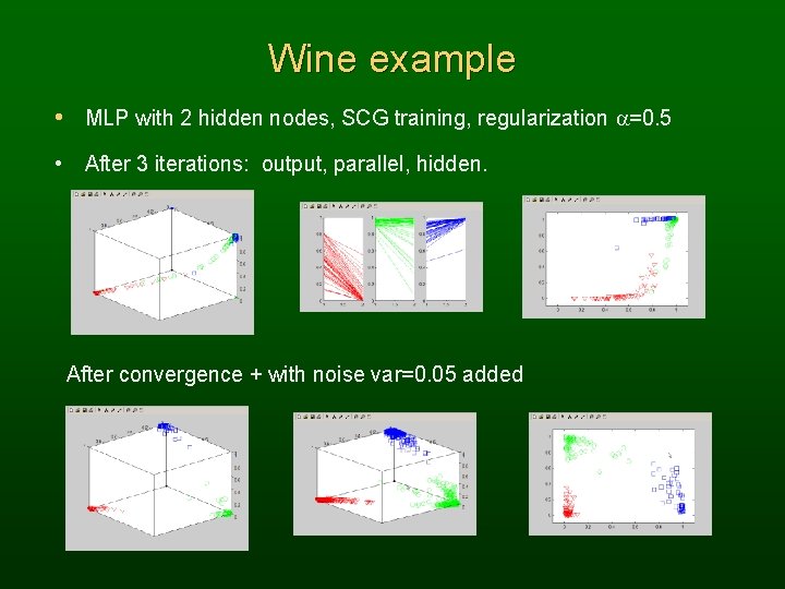
Wine example • MLP with 2 hidden nodes, SCG training, regularization a=0. 5 • After 3 iterations: output, parallel, hidden. After convergence + with noise var=0. 05 added

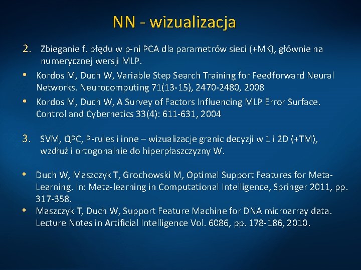
NN - wizualizacja 2. Zbieganie f. błędu w p-ni PCA dla parametrów sieci (+MK), głównie na numerycznej wersji MLP. • Kordos M, Duch W, Variable Step Search Training for Feedforward Neural Networks. Neurocomputing 71(13 -15), 2470 -2480, 2008 • Kordos M, Duch W, A Survey of Factors Influencing MLP Error Surface. Control and Cybernetics 33(4): 611 -631, 2004 3. SVM, QPC, P-rules i inne – wizualizacje granic decyzji w 1 i 2 D (+TM), wzdłuż i ortogonalnie do hiperpłaszczyzny W. • Duch W, Maszczyk T, Grochowski M, Optimal Support Features for Meta- Learning. In: Meta-learning in Computational Intelligence, Springer 2011, pp. 317 -358. • Maszczyk T, Duch W, Support Feature Machine for DNA microarray data. Lecture Notes in Artificial Intelligence Vol. 6086, pp. 178 -186, 2010.

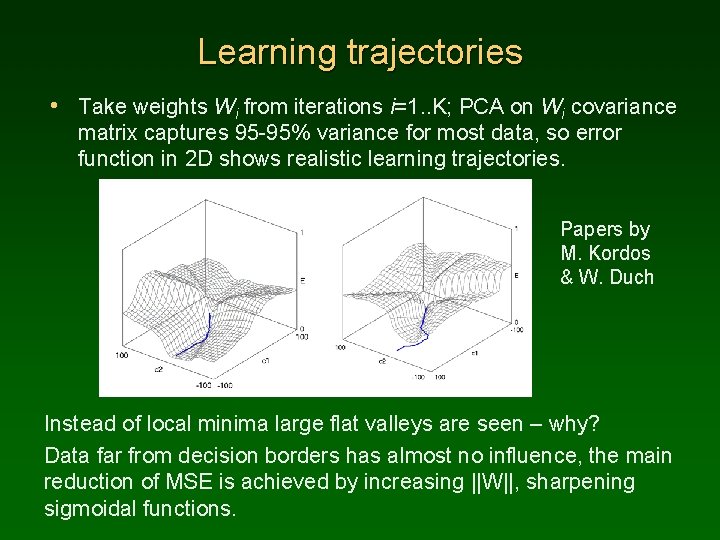
Learning trajectories • Take weights Wi from iterations i=1. . K; PCA on Wi covariance matrix captures 95 -95% variance for most data, so error function in 2 D shows realistic learning trajectories. Papers by M. Kordos & W. Duch Instead of local minima large flat valleys are seen – why? Data far from decision borders has almost no influence, the main reduction of MSE is achieved by increasing ||W||, sharpening sigmoidal functions.

P - rules 35. Probabilistic distance measures for prototype-based rules (PPT 0. 7 MB) Talk presented at the International Conference on Neural Information Processing, ICONIP 2005, Tipei, Taiwan, 1. 11. 2005 60. Computational intelligence for data understanding. Tutorial presented at the BEST 2008 School. Warsaw, Poland, 7. 07, 2008 Więcej: http: //www. is. umk. pl/projects/pbr. html Reguły oparte na prototypach są bardziej ogólne i często łatwiejsze w interpretacji niż reguły rozmyte. F-rules => P-rules, ale nie zawsze P-rules=>F-rules. W szczególności jeśli mamy nieaddytywne funkcje podobieństwa, lub różne metryki probabilistyczne VDM, i inne. FSM to realizacja Separable Function Network.

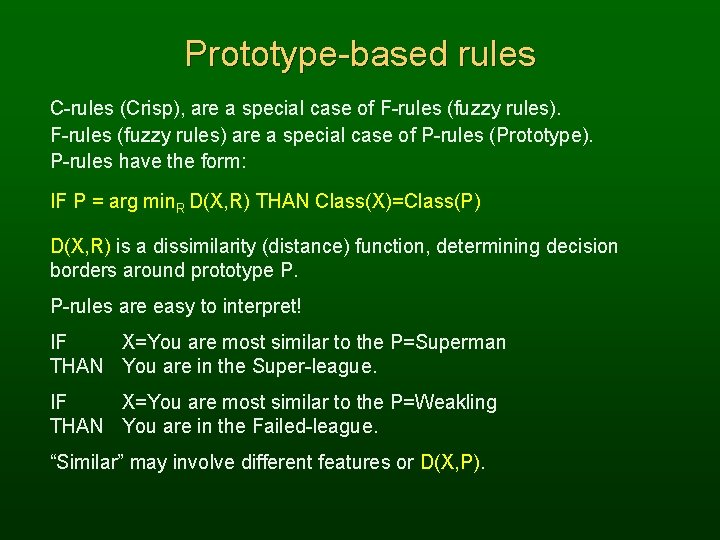
Prototype-based rules C-rules (Crisp), are a special case of F-rules (fuzzy rules) are a special case of P-rules (Prototype). P-rules have the form: IF P = arg min. R D(X, R) THAN Class(X)=Class(P) D(X, R) is a dissimilarity (distance) function, determining decision borders around prototype P. P-rules are easy to interpret! IF X=You are most similar to the P=Superman THAN You are in the Super-league. IF X=You are most similar to the P=Weakling THAN You are in the Failed-league. “Similar” may involve different features or D(X, P).

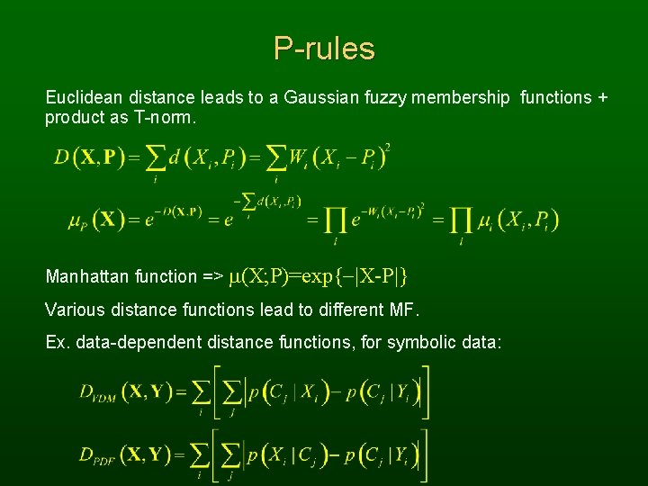
P-rules Euclidean distance leads to a Gaussian fuzzy membership functions + product as T-norm. Manhattan function => m(X; P)=exp{-|X-P|} Various distance functions lead to different MF. Ex. data-dependent distance functions, for symbolic data:

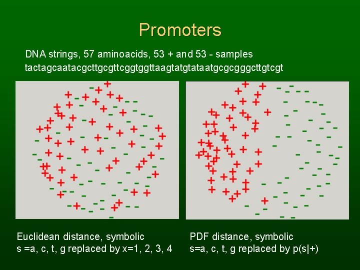
Promoters DNA strings, 57 aminoacids, 53 + and 53 - samples tactagcaatacgcttgcgttcggtggttaagtataatgcgcgggcttgtcgt Euclidean distance, symbolic s =a, c, t, g replaced by x=1, 2, 3, 4 PDF distance, symbolic s=a, c, t, g replaced by p(s|+)

P-rules New distance functions from info theory => interesting MF. MF => new distance function, with local D(X, R) for each cluster. Crisp logic rules: use Chebyshev distance (L norm): DCh(X, P) = ||X-P|| = maxi Wi |Xi-Pi| DCh(X, P) = const => rectangular contours. Chebyshev distance with thresholds P IF DCh(X, P) P THEN C(X)=C(P) is equivalent to a conjunctive crisp rule IF X 1 [P 1 - P/W 1, P 1+ P/W 1] THEN C(X)=C(P) …XN [PN - P/WN, PN+ P/WN]

Decision borders D(P, X)=const and decision borders D(P, X)=D(Q, X). Euclidean distance from 3 prototypes, one per class. Minkovski a=20 distance from 3 prototypes.

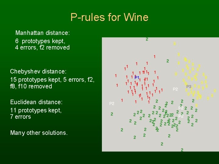
P-rules for Wine Manhattan distance: 6 prototypes kept, 4 errors, f 2 removed Chebyshev distance: 15 prototypes kept, 5 errors, f 2, f 8, f 10 removed Euclidean distance: 11 prototypes kept, 7 errors Many other solutions.

SVNT 31. Support Vector Neural Training (PPT 1137 k. B), ICANN'2005, September 1115, 2005 Duch W, Support Vector Neural Training. Lecture Notes in Computer Science, Vol 3697, 67 -72, 2005

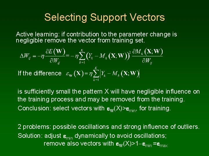
Selecting Support Vectors Active learning: if contribution to the parameter change is negligible remove the vector from training set. If the difference is sufficiently small the pattern X will have negligible influence on the training process and may be removed from the training. Conclusion: select vectors with e. W(X)>emin, for training. 2 problems: possible oscillations and strong influence of outliers. Solution: adjust emin dynamically to avoid oscillations; remove also vectors with e. W(X)>1 -emin =emax

SVNT algorithm Initialize the network parameters W, set De=0. 01, emin=0, set SV=T. Until no improvement is found in the last Nlast iterations do • Optimize network parameters for Nopt steps on SV data. • Run feedforward step on T to determine overall accuracy and errors, take SV={X|e(X) [emin, 1 -emin]}. • If the accuracy increases: compare current network with the previous best one, choose the better one as the current best • increase emin=emin+De and make forward step selecting SVs • If the number of support vectors |SV| increases: decrease emin=emin-De; decrease De = De/1. 2 to avoid large changes

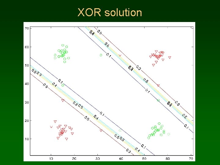
XOR solution

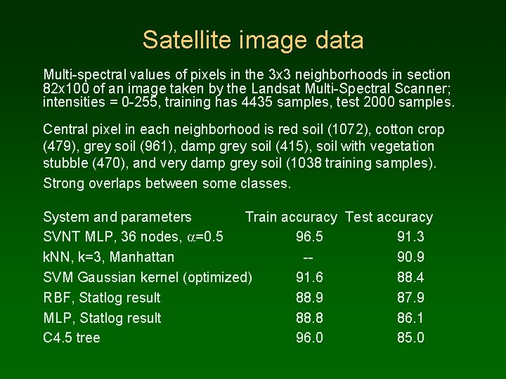
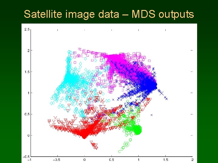
Satellite image data Multi-spectral values of pixels in the 3 x 3 neighborhoods in section 82 x 100 of an image taken by the Landsat Multi-Spectral Scanner; intensities = 0 -255, training has 4435 samples, test 2000 samples. Central pixel in each neighborhood is red soil (1072), cotton crop (479), grey soil (961), damp grey soil (415), soil with vegetation stubble (470), and very damp grey soil (1038 training samples). Strong overlaps between some classes. System and parameters Train accuracy Test accuracy SVNT MLP, 36 nodes, a=0. 5 96. 5 91. 3 k. NN, k=3, Manhattan -90. 9 SVM Gaussian kernel (optimized) 91. 6 88. 4 RBF, Statlog result 88. 9 87. 9 MLP, Statlog result 88. 8 86. 1 C 4. 5 tree 96. 0 85. 0

Satellite image data – MDS outputs

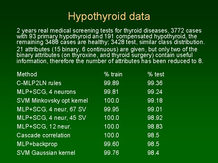
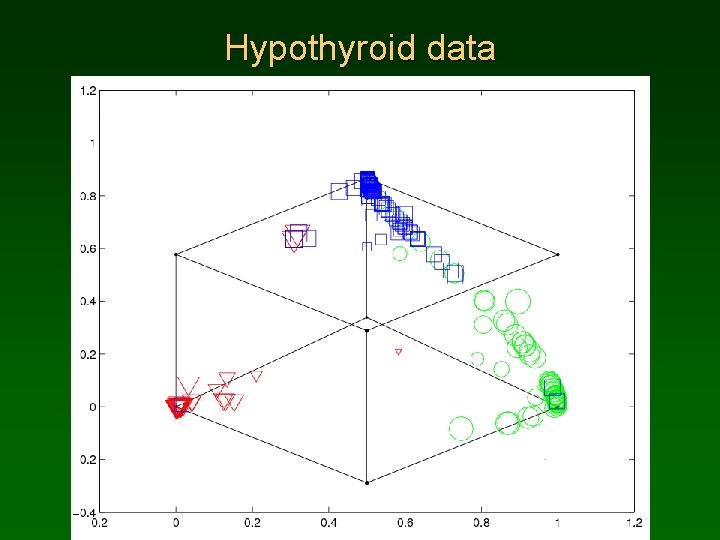
Hypothyroid data 2 years real medical screening tests for thyroid diseases, 3772 cases with 93 primary hypothyroid and 191 compensated hypothyroid, the remaining 3488 cases are healthy; 3428 test, similar class distribution. 21 attributes (15 binary, 6 continuous) are given, but only two of the binary attributes (on thyroxine, and thyroid surgery) contain useful information, therefore the number of attributes has been reduced to 8. Method C-MLP 2 LN rules MLP+SCG, 4 neurons SVM Minkovsky opt kernel MLP+SCG, 4 neur, 67 SV MLP+SCG, 4 neur, 45 SV MLP+SCG, 12 neur. Cascade correlation MLP+backprop SVM Gaussian kernel % train 99. 89 99. 81 100. 0 99. 95 100. 0 99. 60 99. 76 % test 99. 36 99. 24 99. 18 99. 01 98. 92 98. 83 98. 5 98. 4

Hypothyroid data

Discussion SVNT is very easy to implement, here only batch version with SCG training was used. First step only, but promising results. Found smaller support vector sets than SVM; may be useful in one-class learning; speeds up training. Problems: possible oscillations, selection requires more careful analysis – but oscillations help to explore the MSE landscape; additional parameters – but rather easy to set; More empirical tests needed.

NN - uczenie 31. Support Vector Neural Training (PPT 1137 k. B), ICANN'2005, September 11 -15, 2005 74 b. Almost Random Projection Machine with Margin Maximization and Kernel Features (PPTX 1. 0 MB). Presented at: Talk presented at the International Conference on Artificial Neural Networks (ICANN'10), Thessaloniki, Greece, 15. 09. 2010. Paper: Maszczyk T, Duch W, Almost Random Projection Machine with Margin Maximization and Kernel Features. . Lecture Notes in Computer Science Vol. 6353, pp. 40 -48, 2010 Add new kernel feature to ensure wide classification margin.

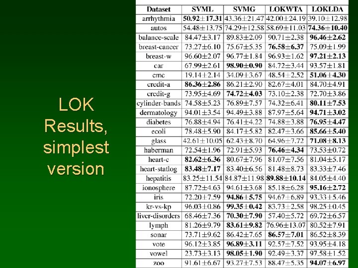
NN - uczenie 31. Support Vector Neural Training (PPT 1137 k. B), ICANN'2005, September 11 -15, 2005 74 b. Almost Random Projection Machine with Margin Maximization and Kernel Features (PPTX 1. 0 MB). Presented at: Talk presented at the International Conference on Artificial Neural Networks (ICANN'10), Thessaloniki, Greece, 15. 09. 2010. Paper: Maszczyk T, Duch W, Almost Random Projection Machine with Margin Maximization and Kernel Features. . Lecture Notes in Computer Science Vol. 6353, pp. 40 -48, 2010 Maszczyk T, Duch W, Locally Optimized Kernels. LNCS 7267, pp. 412– 420, 2012. (ICAISC 2012). Replacing the input space by a kernel-based feature space allows for mixing various kernels and adding new types of features. We show here how to generate locally optimized kernels that facilitate multi-resolution and can handle complex data distributions using simpler models than the standard data formulation may provide.

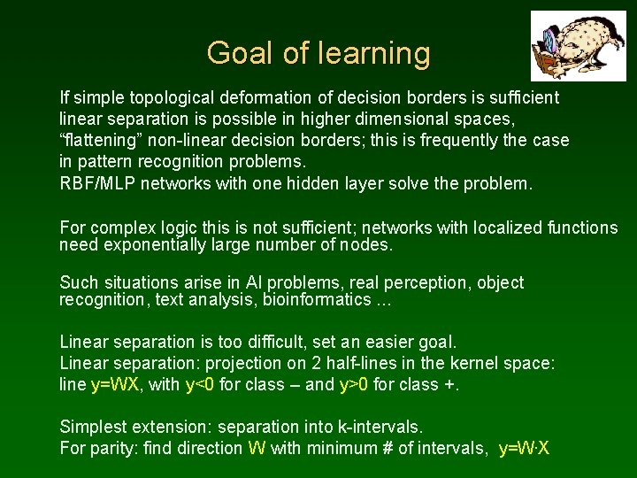
Goal of learning If simple topological deformation of decision borders is sufficient linear separation is possible in higher dimensional spaces, “flattening” non-linear decision borders; this is frequently the case in pattern recognition problems. RBF/MLP networks with one hidden layer solve the problem. For complex logic this is not sufficient; networks with localized functions need exponentially large number of nodes. Such situations arise in AI problems, real perception, object recognition, text analysis, bioinformatics. . . Linear separation is too difficult, set an easier goal. Linear separation: projection on 2 half-lines in the kernel space: line y=WX, with y<0 for class – and y>0 for class +. Simplest extension: separation into k-intervals. For parity: find direction W with minimum # of intervals, y=W. X

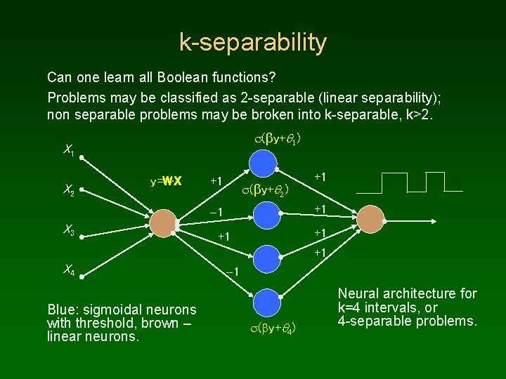
k-separability Can one learn all Boolean functions? Problems may be classified as 2 -separable (linear separability); non separable problems may be broken into k-separable, k>2. s(by+q 1) X 1 X 2 y=W. X +1 s(by+q 2) +1 -1 X 3 +1 +1 X 4 Blue: sigmoidal neurons with threshold, brown – linear neurons. -1 s(by+q 4) Neural architecture for k=4 intervals, or 4 -separable problems.

k-sep learning Try to find lowest k with good solution: • Assume k=2 (linear separability), try to find a good solution; • MSE error criterion • if k=2 is not sufficient, try k=3; two possibilities are C+, C-, C+ and C-, C+, C- this requires only one interval for the middle class; • if k<4 is not sufficient, try k=4; two possibilities are C+, C-, C+, Cand C-, C+, C-, C+ this requires one closed and one open interval. Network solution to minimization of specific cost function. First term = MSE, second penalty for “impure” clusters, third term = reward for the large clusters.

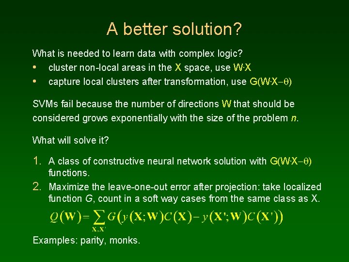
A better solution? What is needed to learn data with complex logic? • cluster non-local areas in the X space, use W. X • capture local clusters after transformation, use G(W. X- ) SVMs fail because the number of directions W that should be considered grows exponentially with the size of the problem n. What will solve it? 1. A class of constructive neural network solution with G(W. X- ) functions. 2. Maximize the leave-one-out error after projection: take localized function G, count in a soft way cases from the same class as X. Examples: parity, monks.

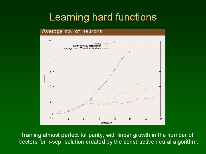
Learning hard functions Training almost perfect for parity, with linear growth in the number of vectors for k-sep. solution created by the constructive neural algorithm.

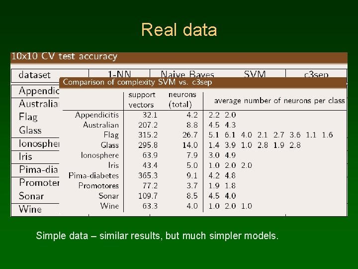
Real data Simple data – similar results, but much simpler models.

Locally Optimized Kernels LOK Algorithm

LOK Results, simplest version

Neurocognitive informatics Use inspirations from the brain, derive practical algorithms! My own attempts - see my webpage, Google: W. Duch 1. Mind as a shadow of neurodynamics: geometrical model of mind processes, psychological spaces providing inner perspective as an approximation to neurodynamics. 2. Intuition: learning from partial observations, solving problems without explicit reasoning (and combinatorial complexity) in an intuitive way. 3. Neurocognitive linguistics: how to find neural pathways in the brain. 4. Creativity in limited domains + word games, good fields for testing. Duch W, Intuition, Insight, Imagination and Creativity, IEEE Computational Intelligence Magazine 2(3), August 2007, pp. 40 -52

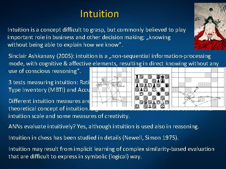
Intuition is a concept difficult to grasp, but commonly believed to play important role in business and other decision making; „knowing without being able to explain how we know”. Sinclair Ashkanasy (2005): intuition is a „non-sequential information-processing mode, with cognitive & affective elements, resulting in direct knowing without any use of conscious reasoning”. 3 tests measuring intuition: Rational-Experiential Inventory (REI), Myers-Briggs Type Inventory (MBTI) and Accumulated Clues Task (ACT). Different intuition measures are not correlated, showing problems in constructing theoretical concept of intuition. Significant correlations were found between REI intuition scale and some measures of creativity. ANNs evaluate intuitively? Yes, although intuition is used also in reasoning. Intuition in chess has been studied in details (Newell, Simon 1975). Intuition may result from implicit learning of complex similarity-based evaluation that are difficult to express in symbolic (logical) way.

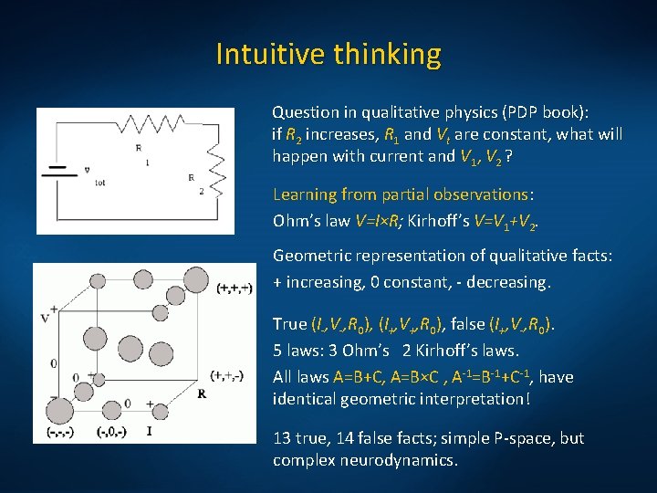
Intuitive thinking Question in qualitative physics (PDP book): if R 2 increases, R 1 and Vt are constant, what will happen with current and V 1, V 2 ? Learning from partial observations: Ohm’s law V=I×R; Kirhoff’s V=V 1+V 2. Geometric representation of qualitative facts: + increasing, 0 constant, - decreasing. True (I-, V-, R 0), (I+, V+, R 0), false (I+, V-, R 0). 5 laws: 3 Ohm’s 2 Kirhoff’s laws. All laws A=B+C, A=B×C , A-1=B-1+C-1, have identical geometric interpretation! 13 true, 14 false facts; simple P-space, but complex neurodynamics.

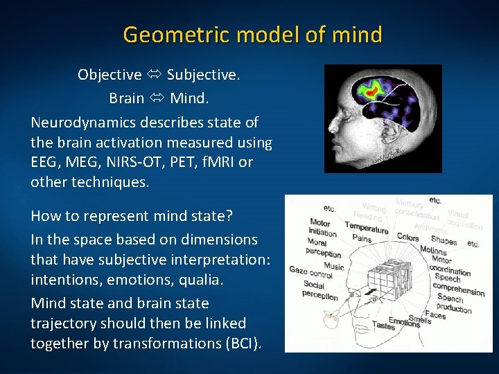
Geometric model of mind Objective Subjective. Brain Mind. Neurodynamics describes state of the brain activation measured using EEG, MEG, NIRS-OT, PET, f. MRI or other techniques. How to represent mind state? In the space based on dimensions that have subjective interpretation: intentions, emotions, qualia. Mind state and brain state trajectory should then be linked together by transformations (BCI).

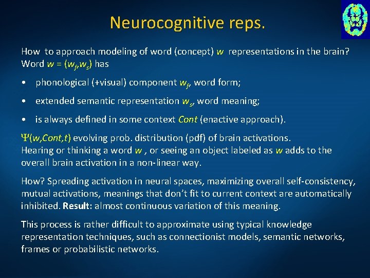
Neurocognitive reps. How to approach modeling of word (concept) w representations in the brain? Word w = (wf, ws) has • phonological (+visual) component wf, word form; • extended semantic representation ws, word meaning; • is always defined in some context Cont (enactive approach). (w, Cont, t) evolving prob. distribution (pdf) of brain activations. Hearing or thinking a word w , or seeing an object labeled as w adds to the overall brain activation in a non-linear way. How? Spreading activation in neural spaces, maximizing overall self-consistency, mutual activations, meanings that don’t fit to current context are automatically inhibited. Result: almost continuous variation of this meaning. This process is rather difficult to approximate using typical knowledge representation techniques, such as connectionist models, semantic networks, frames or probabilistic networks.

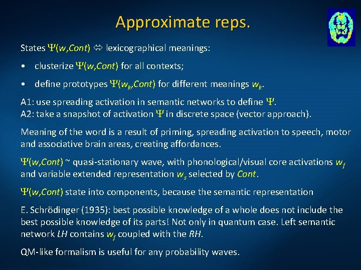
Approximate reps. States (w, Cont) lexicographical meanings: • clusterize (w, Cont) for all contexts; • define prototypes (wk, Cont) for different meanings wk. A 1: use spreading activation in semantic networks to define . A 2: take a snapshot of activation in discrete space (vector approach). Meaning of the word is a result of priming, spreading activation to speech, motor and associative brain areas, creating affordances. (w, Cont) ~ quasi-stationary wave, with phonological/visual core activations wf and variable extended representation ws selected by Cont. (w, Cont) state into components, because the semantic representation E. Schrödinger (1935): best possible knowledge of a whole does not include the best possible knowledge of its parts! Not only in quantum case. Left semantic network LH contains wf coupled with the RH. QM-like formalism is useful for any probability waves.

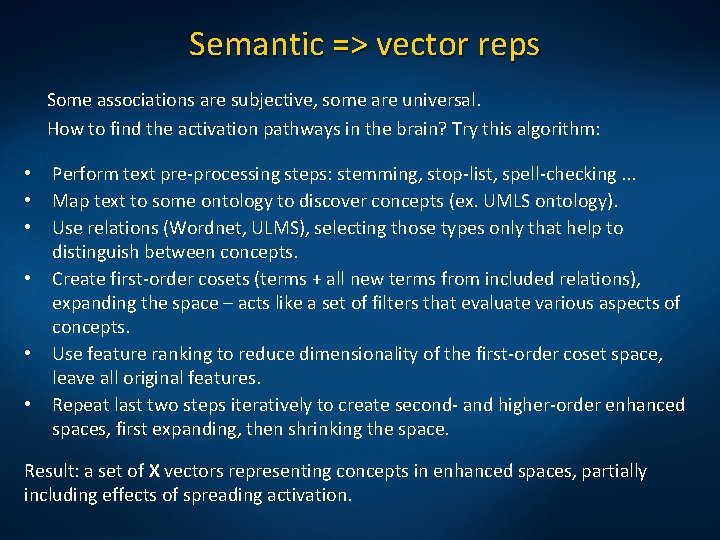
Semantic => vector reps Some associations are subjective, some are universal. How to find the activation pathways in the brain? Try this algorithm: • • • Perform text pre-processing steps: stemming, stop-list, spell-checking. . . Map text to some ontology to discover concepts (ex. UMLS ontology). Use relations (Wordnet, ULMS), selecting those types only that help to distinguish between concepts. Create first-order cosets (terms + all new terms from included relations), expanding the space – acts like a set of filters that evaluate various aspects of concepts. Use feature ranking to reduce dimensionality of the first-order coset space, leave all original features. Repeat last two steps iteratively to create second- and higher-order enhanced spaces, first expanding, then shrinking the space. Result: a set of X vectors representing concepts in enhanced spaces, partially including effects of spreading activation.

Creativity with words The simplest testable model of creativity: • create interesting novel words that capture some features of products; • understand new words that cannot be found in the dictionary. Model inspired by the putative brain processes when new words are being invented starting from some keywords priming auditory cortex. Phonemes (allophones) are resonances, ordered activation of phonemes will activate both known words as well as their combinations; context + inhibition in the winner-takes-most leaves only a few candidate words. Creativity = network+imagination (fluctuations)+filtering (competition) Imagination: chains of phonemes activate both word and non-word representations, depending on the strength of the synaptic connections. Filtering: based on associations, emotions, phonological/semantic density. discoverity = {disc, discover, verity} (discovery, creativity, verity) digventure ={dig, digital, venture, adventure} new! Server: http: //www. braingene. yoyo. pl

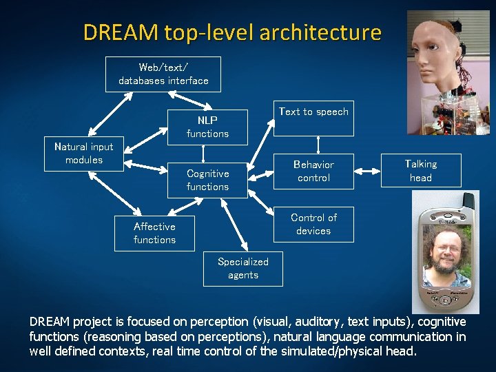
DREAM top-level architecture Web/text/ databases interface NLP functions Natural input modules Cognitive functions Text to speech Behavior control Talking head Control of devices Affective functions Specialized agents DREAM project is focused on perception (visual, auditory, text inputs), cognitive functions (reasoning based on perceptions), natural language communication in well defined contexts, real time control of the simulated/physical head.

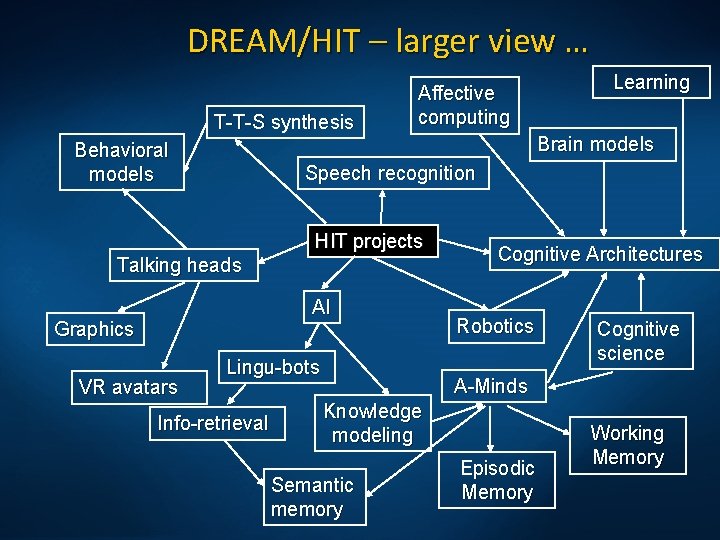
DREAM/HIT – larger view … T-T-S synthesis Behavioral models Affective computing Brain models Speech recognition HIT projects Talking heads AI Graphics VR avatars Learning Lingu-bots Info-retrieval Cognitive Architectures Robotics Cognitive science A-Minds Knowledge modeling Semantic memory Episodic Memory Working Memory