Understanding Medical Data Wodzisaw Duch Department of Informatics

Understanding Medical Data Włodzisław Duch Department of Informatics Nicholas Copernicus University, Toruń, Poland www. phys. uni. torun. pl/~duch

Plan 1. 2. 3. 4. 5. 6. 7. 8. What’s the problem? What we would like to have How to get that Some methods to understand the data Some result Example of applications Expert system for psychometry Conclusions

Department of Computer Methods Computational Intelligence Methods: • neural networks • decision trees • similarity-based methods • visualization Cognitive and Brain Science • theory of mind • modeling human attention Applications • data from psychometrics, medicine, • astronomy, physics, chemistry. . .

with help from. . .

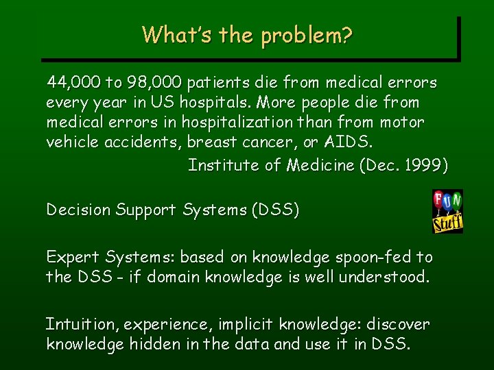
What’s the problem? 44, 000 to 98, 000 patients die from medical errors every year in US hospitals. More people die from medical errors in hospitalization than from motor vehicle accidents, breast cancer, or AIDS. Institute of Medicine (Dec. 1999) Decision Support Systems (DSS) Expert Systems: based on knowledge spoon-fed to the DSS - if domain knowledge is well understood. Intuition, experience, implicit knowledge: discover knowledge hidden in the data and use it in DSS.

What we would like to have Start from good & bad examples evaluated by experts. Understand the data: provide rules; provide prototype cases and similarity measures; provide visualization. Rules should be: simple and/or accurate; reliable and/or general; robust and stable; include alternatives, eliminate improbable.

Logical explanations Logical rules, if simple enough, are usually preferred. • Rules may expose limitations of black box • • methods: statistical, neural or computational intelligence (CI). Only relevant features are used in rules. Rules are sometimes more accurate than NN and other CI methods. Overfitting is easy to control, rules usually have small number of parameters. Rules forever !? • IF the number of rules is relatively small • AND the accuracy is sufficiently high. • THEN rules may be an optimal choice.

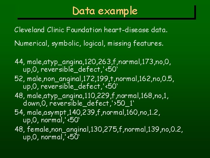
Data example Cleveland Clinic Foundation heart-disease data. Numerical, symbolic, logical, missing features. 44, male, atyp_angina, 120, 263, f, normal, 173, no, 0, up, 0, reversible_defect, '<50‘ 52, male, non_anginal, 172, 199, t, normal, 162, no, 0. 5, up, 0, reversible_defect, '<50‘ 48, male, atyp_angina, 110, 229, f, normal, 168, no, 1, down, 0, reversible_defect, '>50_1‘ 54, male, asympt, 140, 239, f, normal, 160, no, 1. 2, up, 0, normal, '<50‘ 48, female, non_anginal, 130, 275, f, normal, 139, no, 0. 2, up, 0, normal, '<50‘

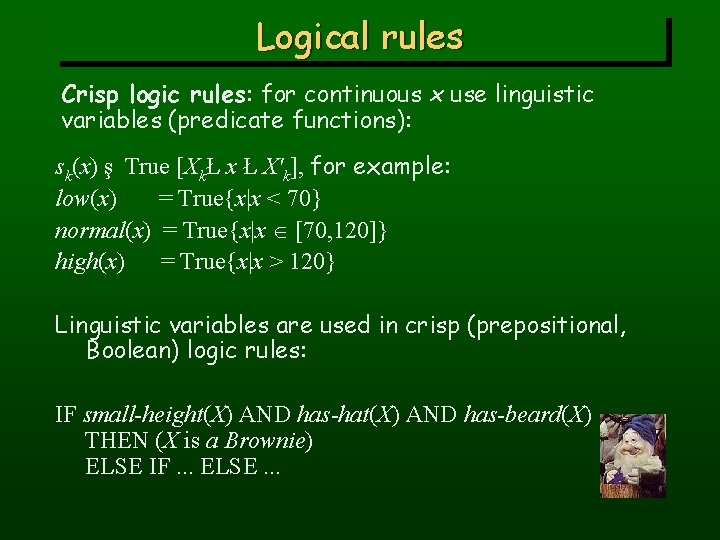
Logical rules Crisp logic rules: for continuous x use linguistic variables (predicate functions): sk(x) ş True [XkŁ x Ł X'k], for example: low(x) = True{x|x < 70} normal(x) = True{x|x [70, 120]} high(x) = True{x|x > 120} Linguistic variables are used in crisp (prepositional, Boolean) logic rules: IF small-height(X) AND has-hat(X) AND has-beard(X) THEN (X is a Brownie) ELSE IF. . . ELSE. . .

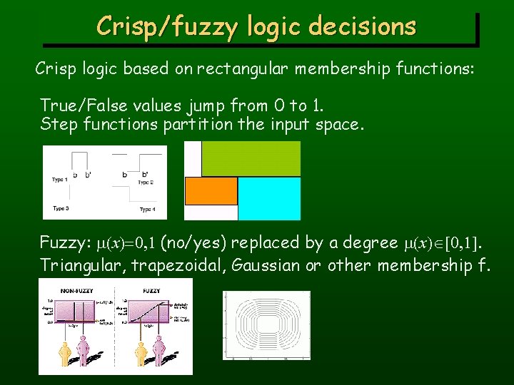
Crisp/fuzzy logic decisions Crisp logic based on rectangular membership functions: True/False values jump from 0 to 1. Step functions partition the input space. Fuzzy: m(x)=0, 1 (no/yes) replaced by a degree m(x) [0, 1]. Triangular, trapezoidal, Gaussian or other membership f.

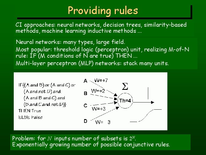
Providing rules CI approaches: neural networks, decision trees, similarity-based methods, machine learning inductive methods. . . Neural networks: many types, large field. Most popular: threshold logic (perceptron) unit, realizing M-of-N rule: IF (M conditions of N are true) THEN. . . Multi-layer perceptron (MLP) networks: stack many units. Problem: for N inputs number of subsets is 2 N. Exponentially growing number of possible conjunctive rules.

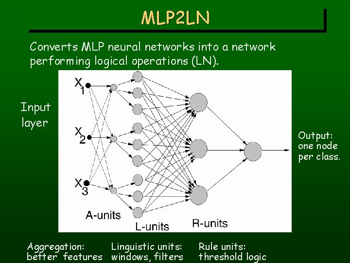
MLP 2 LN Converts MLP neural networks into a network performing logical operations (LN). Input layer Aggregation: Linguistic units: better features windows, filters Output: one node per class. Rule units: threshold logic

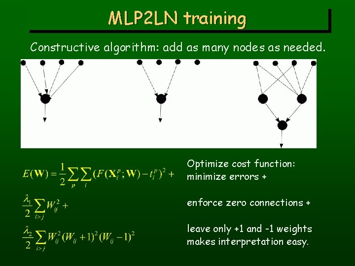
MLP 2 LN training Constructive algorithm: add as many nodes as needed. Optimize cost function: minimize errors + enforce zero connections + leave only +1 and -1 weights makes interpretation easy.

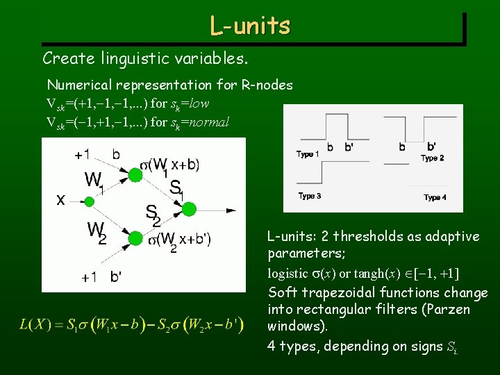
L-units Create linguistic variables. Numerical representation for R-nodes Vsk=(+1, -1, . . . ) for sk=low Vsk=(-1, +1, -1, . . . ) for sk=normal L-units: 2 thresholds as adaptive parameters; logistic s(x) or tangh(x) [-1, +1] Soft trapezoidal functions change into rectangular filters (Parzen windows). 4 types, depending on signs Si.

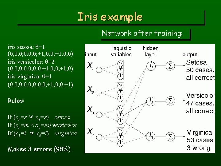
Iris example Network after training: iris setosa: q=1 (0, 0, 0; +1, 0, 0) iris versicolor: q=2 (0, 0, 0; 0, +1, 0) iris virginica: q=1 (0, 0, 0; 0, 0, +1; 0, 0, +1) Rules: If (x 3=s x 4=s) setosa If (x 3=m x 4=m) versicolor If (x 3=l x 4=l) virginica Makes 3 errors (98%).

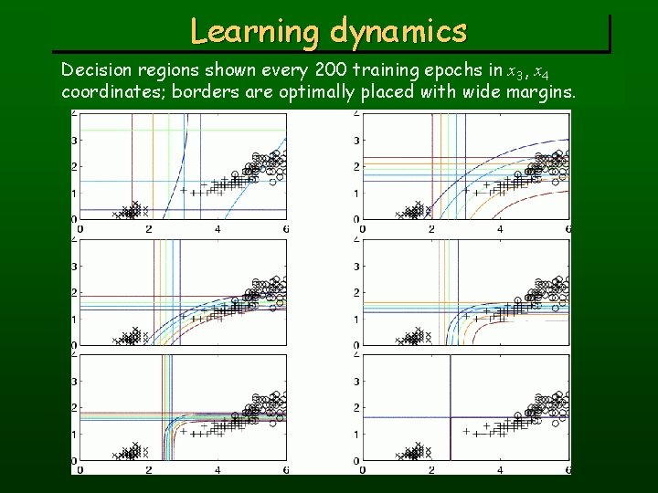
Learning dynamics Decision regions shown every 200 training epochs in x 3, x 4 coordinates; borders are optimally placed with wide margins.

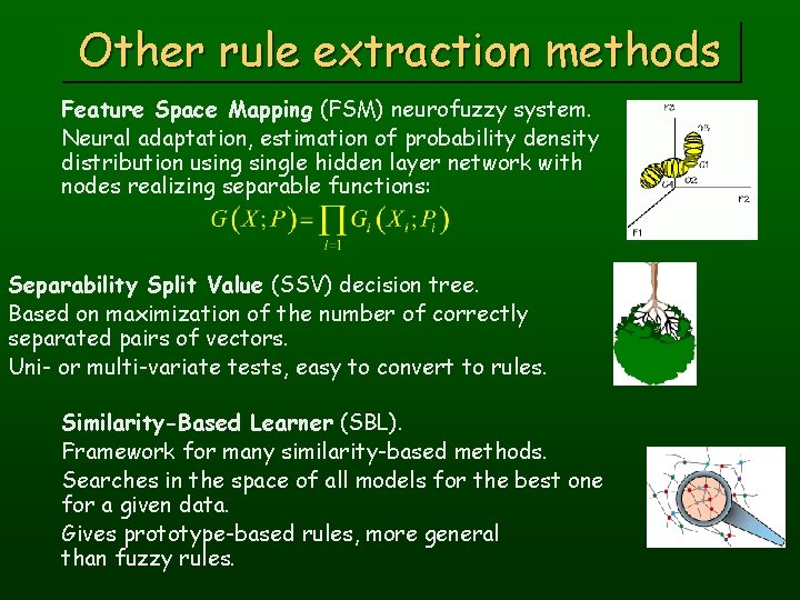
Other rule extraction methods Feature Space Mapping (FSM) neurofuzzy system. Neural adaptation, estimation of probability density distribution usingle hidden layer network with nodes realizing separable functions: Separability Split Value (SSV) decision tree. Based on maximization of the number of correctly separated pairs of vectors. Uni- or multi-variate tests, easy to convert to rules. Similarity-Based Learner (SBL). Framework for many similarity-based methods. Searches in the space of all models for the best one for a given data. Gives prototype-based rules, more general than fuzzy rules.

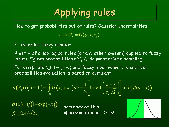
Applying rules How to get probabilities out of rules? Gaussian uncertainties: x - Gaussian fuzzy number. A set R of crisp logical rules (or any other system) applied to fuzzy inputs X gives probabilities p(Ci|X) via Monte Carlo sampling. For crisp rule Ra(x) = {x>a} and fuzzy input value Gx analytical probabilities evaluation is based on cumulant: accuracy of this approximation is < 0. 02

Analytical solution Rule Rab(x) = {x [a, b]} and Gx input has probability: Exact for s(x)(1 - s(x)) error distributions instead of Gaussian. In MLP neural networks: L-units Fuzzy rules + crisp data <=> Crisp rules + fuzzy input Large receptive fields: linguistic variables; small receptive fields: smooth edges. Rules with two or more features in conditions: add probabilities and subtract the overlap:

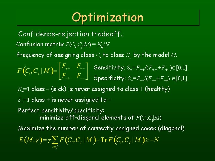
Optimization Confidence-rejection tradeoff. Confusion matrix F(Ci, Cj|M) = Nij/N frequency of assigning class Cj to class Ci by the model M. Sensitivity: S+=F++/(F+++F+-) [0, 1] Specificity: S-=F--/(F--+F-+) [0, 1] S+=1 class - (sick) is never assigned to class + (healthy) S-=1 class + is never assigned to Perfect sensitivity/specificity: minimize off-diagonal elements of F(Ci, Cj|M) Maximize the number of correctly assigned cases (diagonal)

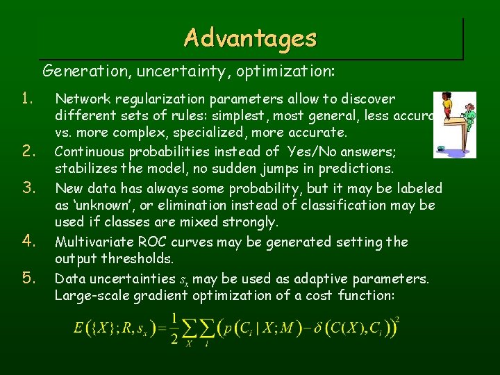
Advantages Generation, uncertainty, optimization: 1. 2. 3. 4. 5. Network regularization parameters allow to discover different sets of rules: simplest, most general, less accurate vs. more complex, specialized, more accurate. Continuous probabilities instead of Yes/No answers; stabilizes the model, no sudden jumps in predictions. New data has always some probability, but it may be labeled as ‘unknown’, or elimination instead of classification may be used if classes are mixed strongly. Multivariate ROC curves may be generated setting the output thresholds. Data uncertainties sx may be used as adaptive parameters. Large-scale gradient optimization of a cost function:

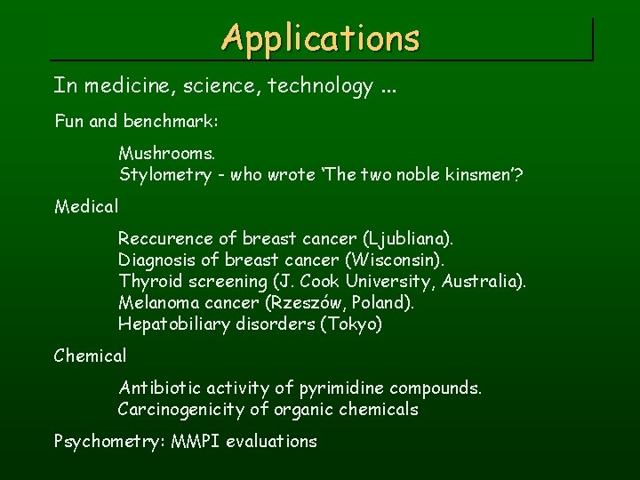
Applications In medicine, science, technology. . . Fun and benchmark: Mushrooms. Stylometry - who wrote ‘The two noble kinsmen’? Medical Reccurence of breast cancer (Ljubliana). Diagnosis of breast cancer (Wisconsin). Thyroid screening (J. Cook University, Australia). Melanoma cancer (Rzeszów, Poland). Hepatobiliary disorders (Tokyo) Chemical Antibiotic activity of pyrimidine compounds. Carcinogenicity of organic chemicals Psychometry: MMPI evaluations

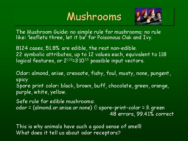
Mushrooms The Mushroom Guide: no simple rule for mushrooms; no rule like: ‘leaflets three, let it be’ for Poisonous Oak and Ivy. 8124 cases, 51. 8% are edible, the rest non-edible. 22 symbolic attributes, up to 12 values each, equivalent to 118 logical features, or 2118=3. 1035 possible input vectors. Odor: almond, anise, creosote, fishy, foul, musty, none, pungent, spicy Spore print color: black, brown, buff, chocolate, green, orange, purple, white, yellow. Safe rule for edible mushrooms: odor = (almond. or. anise. or. none) Ů spore-print-color = Ř green 48 errors, 99. 41% correct This is why animals have such a good sense of smell! What does it tell us about odor receptors?

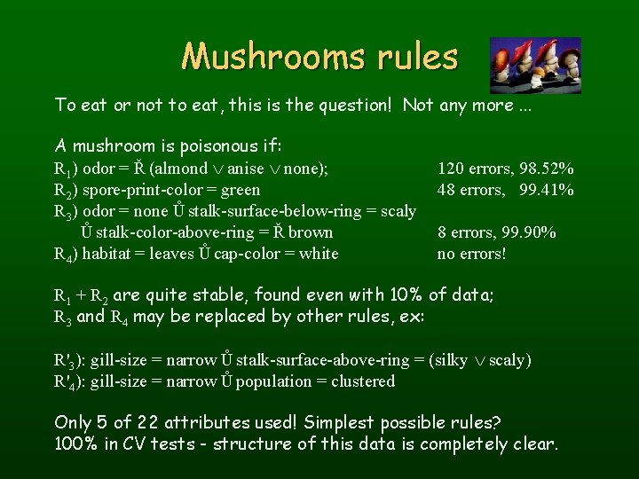
Mushrooms rules To eat or not to eat, this is the question! Not any more. . . A mushroom is poisonous if: R 1) odor = Ř (almond Ú anise Ú none); R 2) spore-print-color = green R 3) odor = none Ů stalk-surface-below-ring = scaly Ů stalk-color-above-ring = Ř brown R 4) habitat = leaves Ů cap-color = white 120 errors, 98. 52% 48 errors, 99. 41% 8 errors, 99. 90% no errors! R 1 + R 2 are quite stable, found even with 10% of data; R 3 and R 4 may be replaced by other rules, ex: R'3): gill-size = narrow Ů stalk-surface-above-ring = (silky Ú scaly) R'4): gill-size = narrow Ů population = clustered Only 5 of 22 attributes used! Simplest possible rules? 100% in CV tests - structure of this data is completely clear.

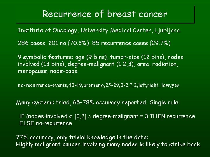
Recurrence of breast cancer Institute of Oncology, University Medical Center, Ljubljana. 286 cases, 201 no (70. 3%), 85 recurrence cases (29. 7%) 9 symbolic features: age (9 bins), tumor-size (12 bins), nodes involved (13 bins), degree-malignant (1, 2, 3), area, radiation, menopause, node-caps. no-recurrence-events, 40 -49, premeno, 25 -29, 0 -2, ? , 2, left, right_low, yes Many systems tried, 65 -78% accuracy reported. Single rule: IF (nodes-involved [0, 2] degree-malignant = 3 THEN recurrence ELSE no-recurrence 77% accuracy, only trivial knowledge in the data: Highly malignant cancer involving many nodes is likely to strike back.

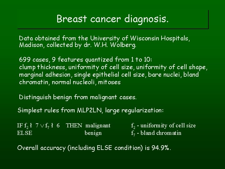
Breast cancer diagnosis. Data obtained from the University of Wisconsin Hospitals, Madison, collected by dr. W. H. Wolberg. 699 cases, 9 features quantized from 1 to 10: clump thickness, uniformity of cell size, uniformity of cell shape, marginal adhesion, single epithelial cell size, bare nuclei, bland chromatin, normal nucleoli, mitoses Distinguish benign from malignant cases. Simplest rules from MLP 2 LN, large regularization: IF f 2 ł 7 Ú f 7 ł 6 ELSE THEN malignant benign f 2 - uniformity of cell size f 7 - bland chromatin Overall accuracy (including ELSE condition) is 94. 9%.

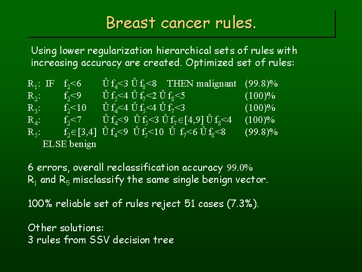
Breast cancer rules. Using lower regularization hierarchical sets of rules with increasing accuracy are created. Optimized set of rules: R 1: IF f 2<6 R 2: f 2<9 R 3: f 2<10 R 4: f 2<7 R 5: f 2 [3, 4] ELSE benign Ů f 4<3 Ů f 8<8 THEN malignant Ů f 5<4 Ů f 7<2 Ů f 8<5 Ů f 4<4 Ů f 5<4 Ů f 7<3 Ů f 4<9 Ů f 5<3 Ů f 7 [4, 9] Ů f 8<4 Ů f 4<9 Ů f 5<10 Ů f 7<6 Ů f 8<8 (99. 8)% (100)% (99. 8)% 6 errors, overall reclassification accuracy 99. 0% R 1 and R 5 misclassify the same single benign vector. 100% reliable set of rules reject 51 cases (7. 3%). Other solutions: 3 rules from SSV decision tree

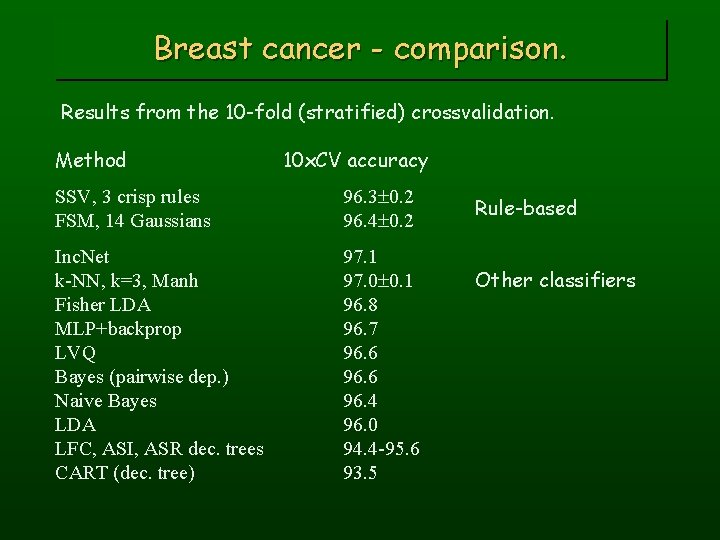
Breast cancer - comparison. Results from the 10 -fold (stratified) crossvalidation. Method 10 x. CV accuracy SSV, 3 crisp rules FSM, 14 Gaussians 96. 3 0. 2 96. 4 0. 2 Inc. Net k-NN, k=3, Manh Fisher LDA MLP+backprop LVQ Bayes (pairwise dep. ) Naive Bayes LDA LFC, ASI, ASR dec. trees CART (dec. tree) 97. 1 97. 0 0. 1 96. 8 96. 7 96. 6 96. 4 96. 0 94. 4 -95. 6 93. 5 Rule-based Other classifiers

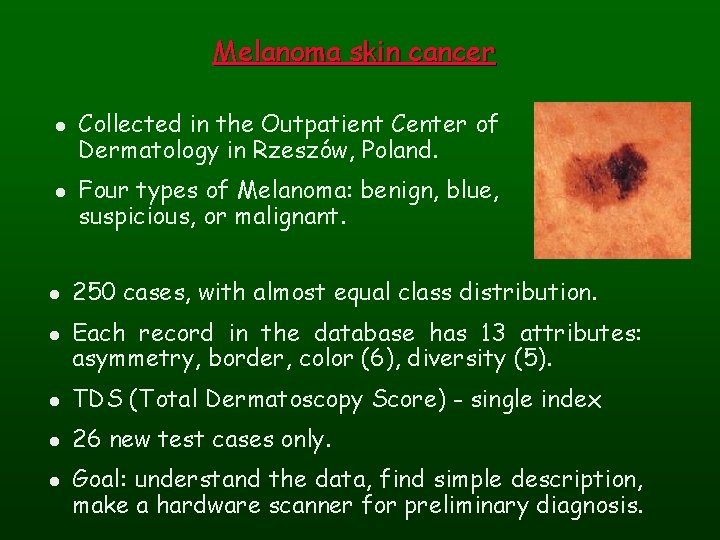
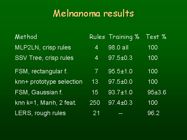
Melanoma skin cancer l l Collected in the Outpatient Center of Dermatology in Rzeszów, Poland. Four types of Melanoma: benign, blue, suspicious, or malignant. 250 cases, with almost equal class distribution. Each record in the database has 13 attributes: asymmetry, border, color (6), diversity (5). l TDS (Total Dermatoscopy Score) - single index l 26 new test cases only. l Goal: understand the data, find simple description, make a hardware scanner for preliminary diagnosis.

Melnanoma results Method Rules Training % Test % MLP 2 LN, crisp rules 4 98. 0 all 100 SSV Tree, crisp rules 4 97. 5± 0. 3 100 FSM, rectangular f. 7 95. 5± 1. 0 100 knn+ prototype selection 13 97. 5± 0. 0 100 FSM, Gaussian f. 15 93. 7± 1. 0 95± 3. 6 knn k=1, Manh, 2 feat. 250 97. 4± 0. 3 100 21 -- 96. 2 LERS, rough rules

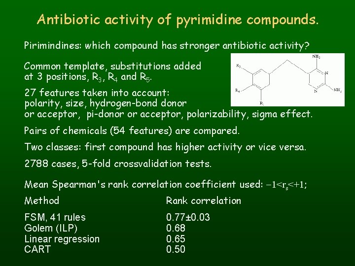
Antibiotic activity of pyrimidine compounds. Pirimindines: which compound has stronger antibiotic activity? Common template, substitutions added at 3 positions, R 3, R 4 and R 5. 27 features taken into account: polarity, size, hydrogen-bond donor or acceptor, pi-donor or acceptor, polarizability, sigma effect. Pairs of chemicals (54 features) are compared. Two classes: first compound has higher activity or vice versa. 2788 cases, 5 -fold crossvalidation tests. Mean Spearman's rank correlation coefficient used: -1<rs<+1; Method Rank correlation FSM, 41 rules Golem (ILP) Linear regression CART 0. 77± 0. 03 0. 68 0. 65 0. 50

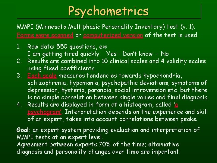
Psychometrics MMPI (Minnesota Multiphasic Personality Inventory) test (v. 1). Forms were scanned or computerized version of the test is used. 1. Row data: 550 questions, ex: I am getting tired quickly Yes - Don’t know - No 2. Results are combined into 10 clinical scales and 4 validity scales using fixed coefficients. 3. Each scale measures tendencies towards hypochondria, schizophrenia, hypomania, psychopathic deviations, symptoms of depression, hysteria, paranoia, social introversion etc, but there is no simple correlation between single values and final diagnosis. 4. Results are displayed in form of a histogram, called ‘a psychogram’. Interpretation depends on the experience and skill of an expert, takes into account correlations between peaks. Goal: an expert system providing evaluation and interpretation of MMPI tests at an expert level. Agreement between experts 70% of the time; alternative diagnosis and personality changes over time are important.

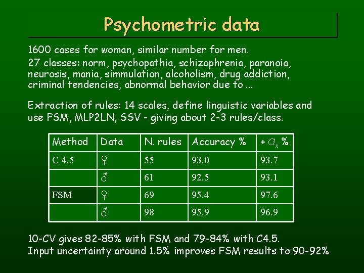
Psychometric data 1600 cases for woman, similar number for men. 27 classes: norm, psychopathia, schizophrenia, paranoia, neurosis, mania, simmulation, alcoholism, drug addiction, criminal tendencies, abnormal behavior due to. . . Extraction of rules: 14 scales, define linguistic variables and use FSM, MLP 2 LN, SSV - giving about 2 -3 rules/class. Method Data N. rules Accuracy % + Gx % C 4. 5 ♀ 55 93. 0 93. 7 ♂ 61 92. 5 93. 1 ♀ 69 95. 4 97. 6 ♂ 98 95. 9 96. 9 FSM 10 -CV gives 82 -85% with FSM and 79 -84% with C 4. 5. Input uncertainty around 1. 5% improves FSM results to 90 -92%

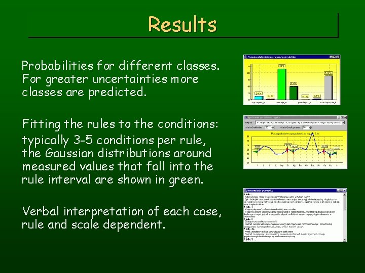
Results Probabilities for different classes. For greater uncertainties more classes are predicted. Fitting the rules to the conditions: typically 3 -5 conditions per rule, the Gaussian distributions around measured values that fall into the rule interval are shown in green. Verbal interpretation of each case, rule and scale dependent.

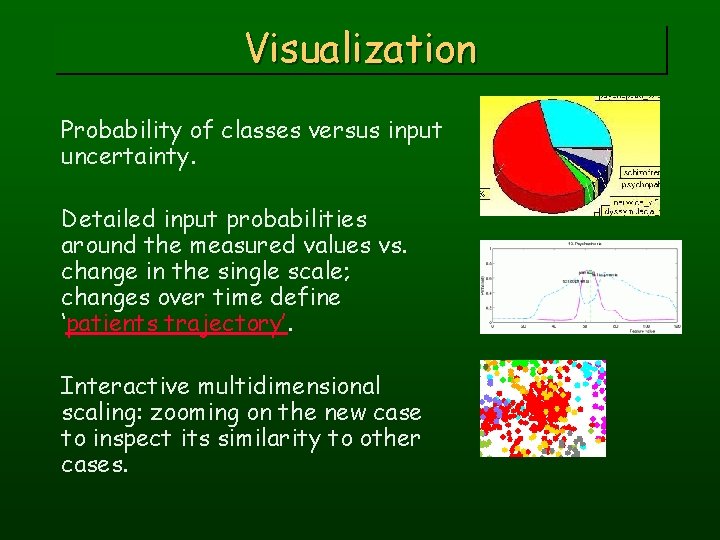
Visualization Probability of classes versus input uncertainty. Detailed input probabilities around the measured values vs. change in the single scale; changes over time define ‘patients trajectory’. Interactive multidimensional scaling: zooming on the new case to inspect its similarity to other cases.

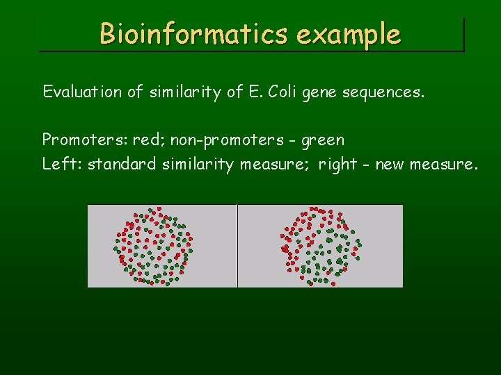
Bioinformatics example Evaluation of similarity of E. Coli gene sequences. Promoters: red; non-promoters - green Left: standard similarity measure; right - new measure.

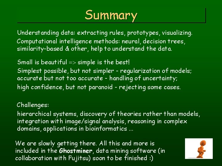
Summary Understanding data: extracting rules, prototypes, visualizing. Computational intelligence methods: neural, decision trees, similarity-based & other, help to understand the data. Small is beautiful => simple is the best! Simplest possible, but not simpler - regularization of models; accurate but not too accurate - handling of uncertainty; high confidence, but not paranoid - rejecting some cases. Challenges: hierarchical systems, discovery of theories rather than models, integration with image/signal analysis, reasoning in complex domains, applications in bioinformatics. . . We are slowly getting there. All this and more is included in the Ghostminer, data mining software (in collaboration with Fujitsu) soon to be finished : )

References IEEE Transactions on Neural Networks 12 (2001) 277 -306 (March issue) www. phys. uni. torun. pl/~duch paper archive