New Newtonian Alchemy Turning Noise into Signal Peter

New Newtonian Alchemy: Turning Noise into Signal Peter Cox Mathematics Research Institute University of Exeter With thanks especially to Chris Huntingford, Ben Booth, Roddy Dewar, Tim Lenton

Outline Ø Maximum Entropy Production – applications to surface-to-atmosphere turbulent fluxes. Ø Interannual variability of CO 2 as a constraint on the sensitivity of tropical land carbon to climate change Ø Amazon Forest Dieback as a Climate Tipping Point – Time-series Precursors ?

Maximum Entropy Production – Applications to Climate (Dewar, Niven, Jupp, Gregory)

Maximum Entropy Production : Application to the Climate System Ø 1960 s : Ed Lorenz suggests that the climate system maximises “work”. (E. Lorenz, 1960) Ø 1970 s : Garth Paltridge develops successful climate model based on the assumption that heat transports maximise the rate of entropy production. (Paltridge 1975; 1978) Ø 2003 : Ralph Lorenz et al. show that MEP is consistent with the observed equator-to-pole temperature contrasts on Titan and Mars (as well as Earth). (R. Lorenz et al. , 2003).

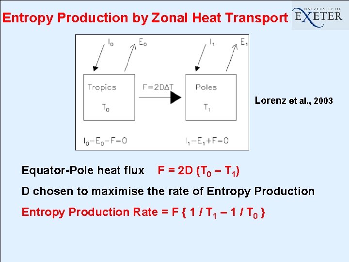
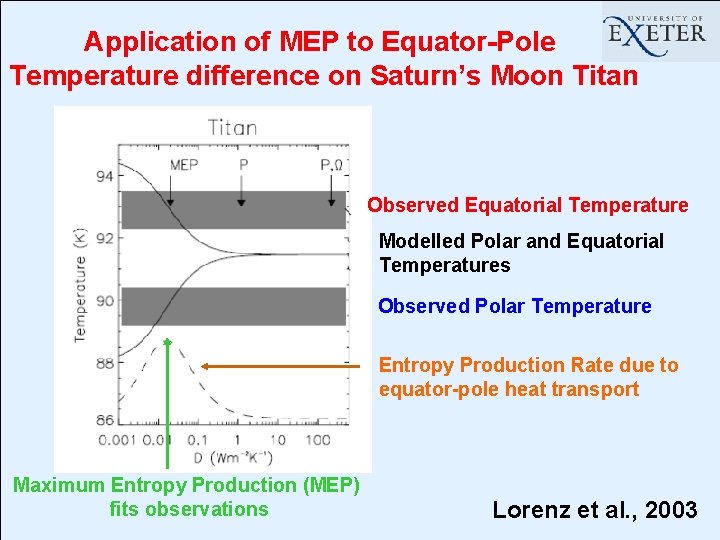
Entropy Production by Zonal Heat Transport Lorenz et al. , 2003 Equator-Pole heat flux F = 2 D (T 0 – T 1) D chosen to maximise the rate of Entropy Production Rate = F { 1 / T 1 – 1 / T 0 }

Application of MEP to Equator-Pole Temperature difference on Saturn’s Moon Titan Observed Equatorial Temperature Modelled Polar and Equatorial Temperatures Observed Polar Temperature Entropy Production Rate due to equator-pole heat transport Maximum Entropy Production (MEP) fits observations Lorenz et al. , 2003

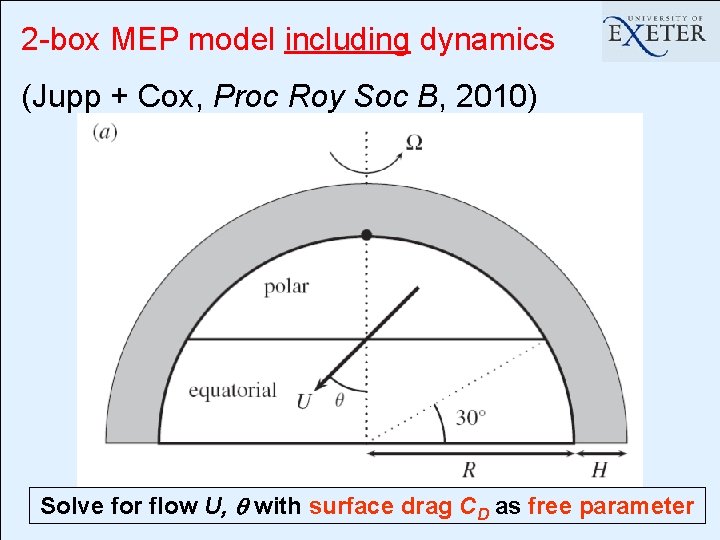
2 -box MEP model including dynamics (Jupp + Cox, Proc Roy Soc B, 2010) Solve for flow U, q with surface drag CD as free parameter

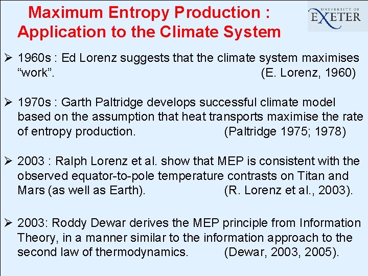
Maximum Entropy Production : Application to the Climate System Ø 1960 s : Ed Lorenz suggests that the climate system maximises “work”. (E. Lorenz, 1960) Ø 1970 s : Garth Paltridge develops successful climate model based on the assumption that heat transports maximise the rate of entropy production. (Paltridge 1975; 1978) Ø 2003 : Ralph Lorenz et al. show that MEP is consistent with the observed equator-to-pole temperature contrasts on Titan and Mars (as well as Earth). (R. Lorenz et al. , 2003). Ø 2003: Roddy Dewar derives the MEP principle from Information Theory, in a manner similar to the information approach to the second law of thermodynamics. (Dewar, 2003, 2005).

“Dangerously Seductive”. . . but sometimes it’s nice to be seduced. . .

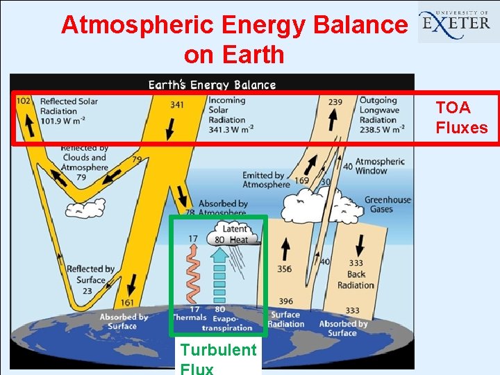
Atmospheric Energy Balance on Earth TOA Fluxes Turbulent

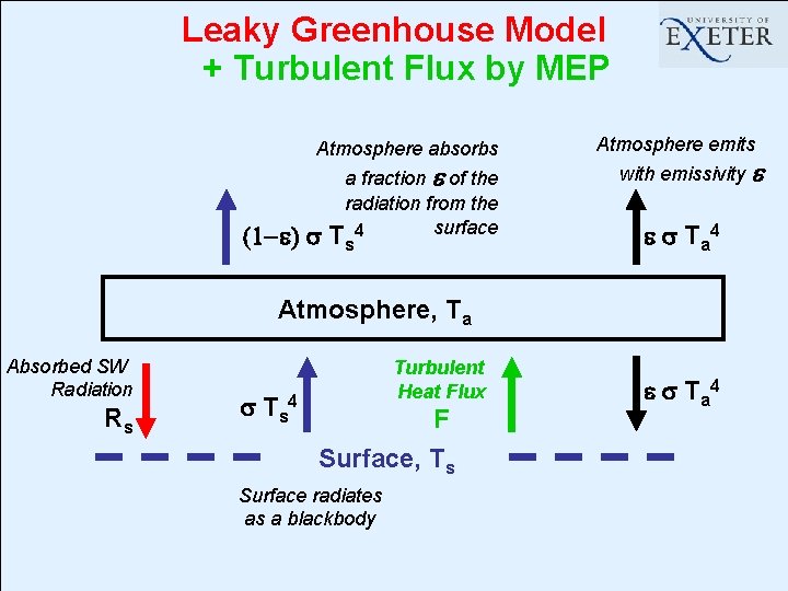
Leaky Greenhouse Model + Turbulent Flux by MEP Atmosphere absorbs a fraction e of the radiation from the surface 4 (1 -e) s Ts Atmosphere emits with emissivity e e s T a 4 Atmosphere, Ta Absorbed SW Radiation Rs Turbulent Heat Flux s T s 4 F Surface, Ts Surface radiates as a blackbody e s T a 4

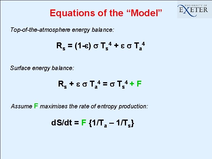
Equations of the “Model” Top-of-the-atmosphere energy balance: Rs = (1 -e) s Ts 4 + e s Ta 4 Surface energy balance: R s + e s T a 4 = s T s 4 + F Assume F maximises the rate of entropy production: d. S/dt = F {1/Ta – 1/Ts}

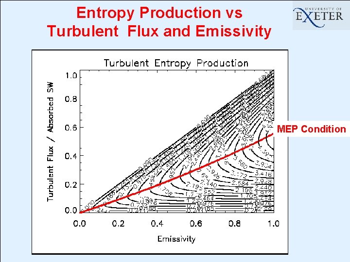
Entropy Production vs Turbulent Flux and Emissivity MEP Condition

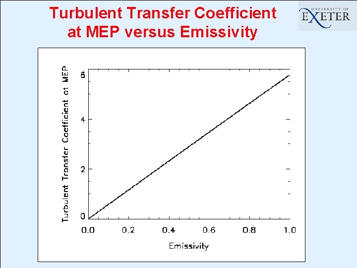
Turbulent Transfer Coefficient at MEP versus Emissivity

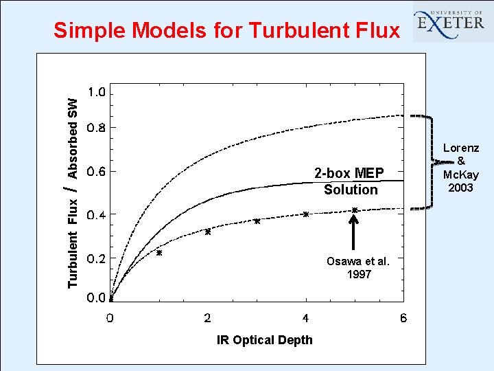
Absorbed SW Simple Models for Turbulent Flux / 2 -box MEP Solution Osawa et al. 1997 IR Optical Depth Lorenz & Mc. Kay 2003

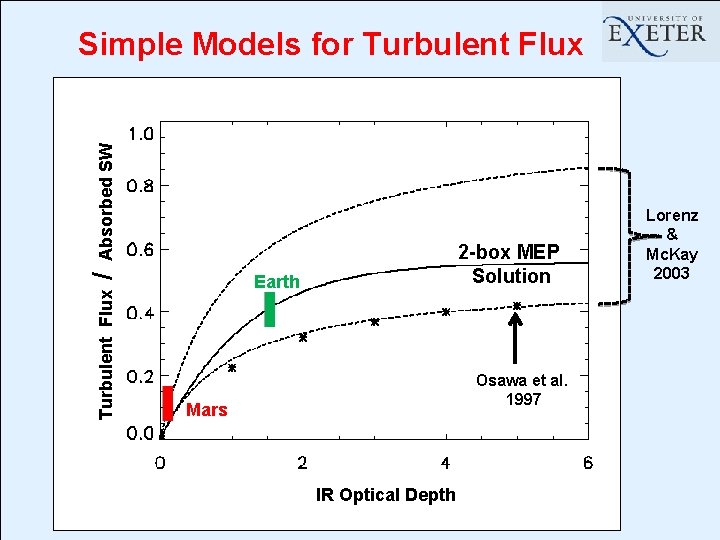
Absorbed SW Simple Models for Turbulent Flux Earth / Turbulent Flux 2 -box MEP Solution Osawa et al. 1997 Mars IR Optical Depth Lorenz & Mc. Kay 2003

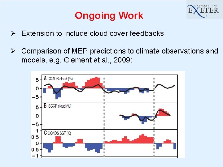
Ongoing Work Ø Extension to include cloud cover feedbacks Ø Comparison of MEP predictions to climate observations and models, e. g. Clement et al. , 2009:

Modelled Climate-Carbon Cycle Feedbacks

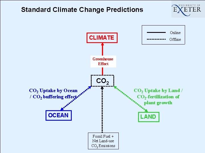
Standard Climate Change Predictions Online CLIMATE Offline Greenhouse Effect CO 2 Uptake by Ocean / CO 2 buffering effect CO 2 Uptake by Land / CO 2 -fertilization of plant growth OCEAN LAND Fossil Fuel + Net Land-use CO 2 Emissions

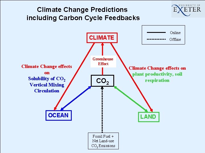
Climate Change Predictions including Carbon Cycle Feedbacks Online CLIMATE Climate Change effects on Solubility of CO 2 Vertical Mixing Circulation Greenhouse Effect CO 2 OCEAN Offline Climate Change effects on plant productivity, soil respiration LAND Fossil Fuel + Net Land-use CO 2 Emissions

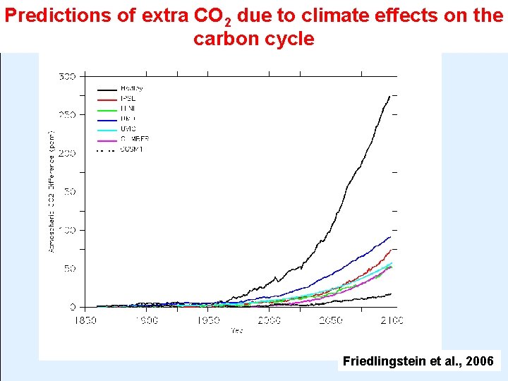
Predictions of extra CO 2 due to climate effects on the carbon cycle Friedlingstein et al. , 2006

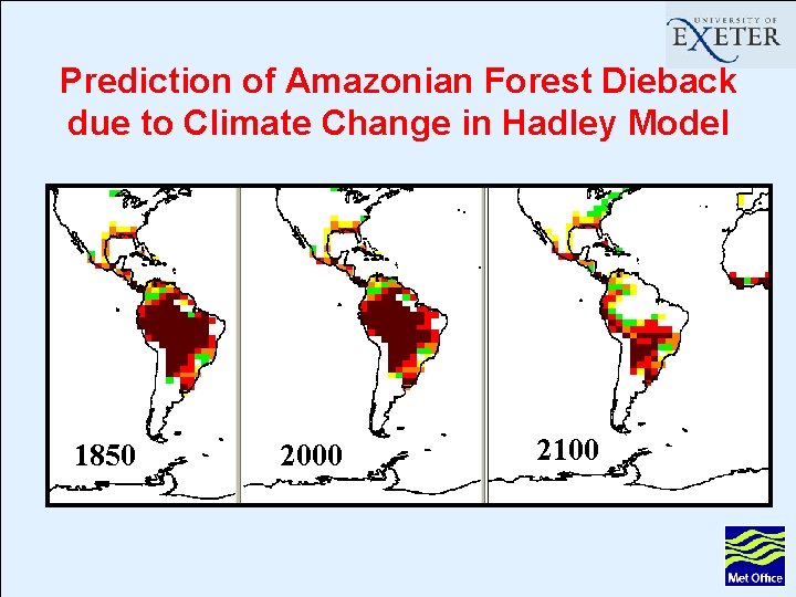
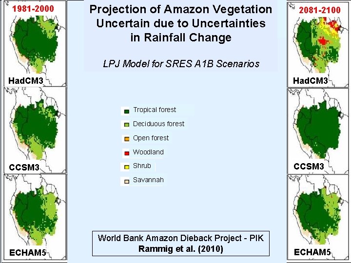
Prediction of Amazonian Forest Dieback due to Climate Change in Hadley Model 1850 2000 2100

1981 -2000 Projection of Amazon Vegetation Uncertain due to Uncertainties in Rainfall Change 2081 -2100 LPJ Model for SRES A 1 B Scenarios Had. CM 3 Tropical forest Deciduous forest Open forest Woodland CCSM 3 Shrub CCSM 3 Savannah ECHAM 5 World Bank Amazon Dieback Project - PIK Rammig et al. (2010) ECHAM 5

Observed Changes in the Carbon Cycle (Global Carbon Project)

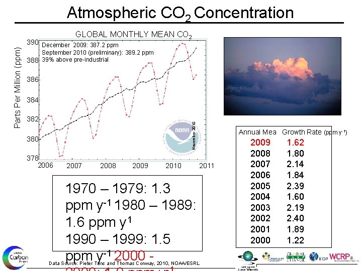
Atmospheric CO 2 Concentration 390 December 2009: 387. 2 ppm September 2010 (preliminary): 389. 2 ppm 388 39% above pre-industrial 386 384 382 November 2010 Parts Per Million (ppm) GLOBAL MONTHLY MEAN CO 2 380 378 2006 2007 2008 2009 2010 1970 – 1979: 1. 3 ppm y-1 1980 – 1989: 1. 6 ppm y 1 1990 – 1999: 1. 5 ppm y-1 2000 - Annual Mea Growth Rate (ppm y-1) 2011 Data Source: Pieter Tans and Thomas Conway, 2010, NOAA/ESRL 2009 2008 2007 2006 2005 2004 2003 2002 2001 2000 1. 62 1. 80 2. 14 1. 84 2. 39 1. 60 2. 19 2. 40 1. 89 1. 22

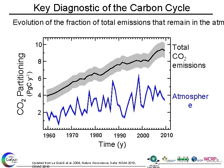
Key Diagnostic of the Carbon Cycle Evolution of the fraction of total emissions that remain in the atm Total CO 2 emissions 8 (Pg. C y-1) CO 2 Partitioning 10 6 4 Atmospher e 2 1960 1970 1980 1990 Time (y) Updated from Le Quéré et al. 2009, Nature Geoscience; Data: NOAA 2010, CDIAC 2010 2000 2010

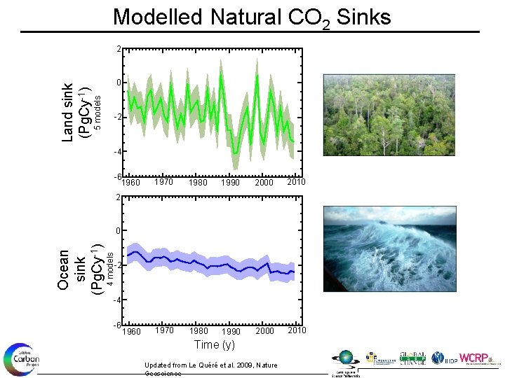
Modelled Natural CO 2 Sinks 0 5 models Land sink (Pg. Cy-1) 2 -2 -4 -6 1960 1970 1980 1990 2000 2010 2 4 models Ocean sink (Pg. Cy-1) 0 -2 -4 -6 1960 Time (y) Updated from Le Quéré et al. 2009, Nature Geoscience

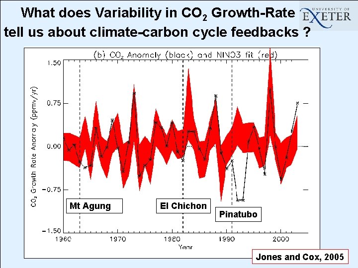
What does Variability in CO 2 Growth-Rate tell us about climate-carbon cycle feedbacks ? 2003 Anomaly Total Fossil Fuels Land-use Change Mt Agung El Chichon Years after Volcanic Eruptions Pinatubo Jones and Cox, 2005

Interannual variability of CO 2 as a constraint on the sensitivity of tropical land carbon to climate change (Booth, Huntingford)

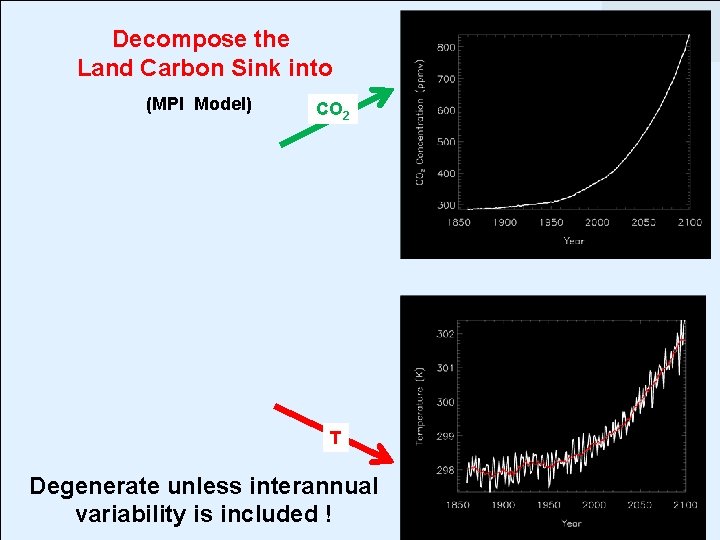
Decompose the Land Carbon Sink into (MPI Model) CO 2 T Degenerate unless interannual variability is included !

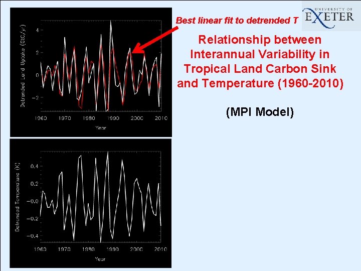
Best linear fit to detrended T Relationship between Interannual Variability in Tropical Land Carbon Sink and Temperature (1960 -2010) (MPI Model)

Residual Trend is assumed to be due to CO 2 fertilization (MPI Model) Good fit to logarithmic dependence on CO 2

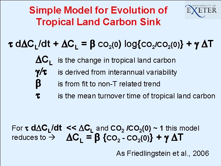
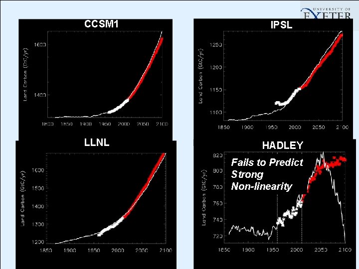
Simple Model for Evolution of Tropical Land Carbon Sink t d. DCL/dt + DCL = b CO 2(0) log{CO 2/CO 2(0)} + g DT DCL g/t b t is the change in tropical land carbon is derived from interannual variability is from fit to non-T related trend is the mean turnover time of tropical land carbon For t d. DCL/dt << DCL and CO 2 /CO 2(0) ~ 1 this model reduces to DCL = b {CO 2 - CO 2(0)} + g DT As Friedlingstein et al. , 2006

Simple Model fit to GCM (MPI) - Tropical Land Carbon Sink Period of Fit

Simple Model fit to GCM (MPI) - Change in Tropical Land Carbon

CCSM 1 LLNL IPSL HADLEY Fails to Predict Strong Non-linearity

Ongoing Work Ø Extension of simple model to capture non-linearities. Ø Estimation of climate impacts on tropical land carbon from the Mauna Loa CO 2 record. Ø Constraints of climate-carbon cycle model projections.

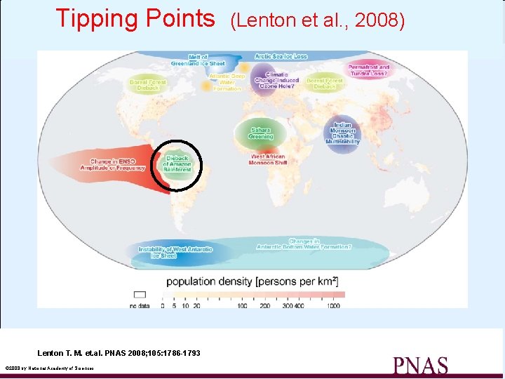
Amazon Forest Dieback as a Climate Tipping Point – Time-series Precursors ? (Huntingford, Lenton, Vitolo)

Tipping Points (Lenton et al. , 2008) Map of potential policy-relevant tipping elements in the climate system, updated from ref. 5 and overlain on global population density Lenton T. M. et. al. PNAS 2008; 105: 1786 -1793 © 2008 by National Academy of Sciences

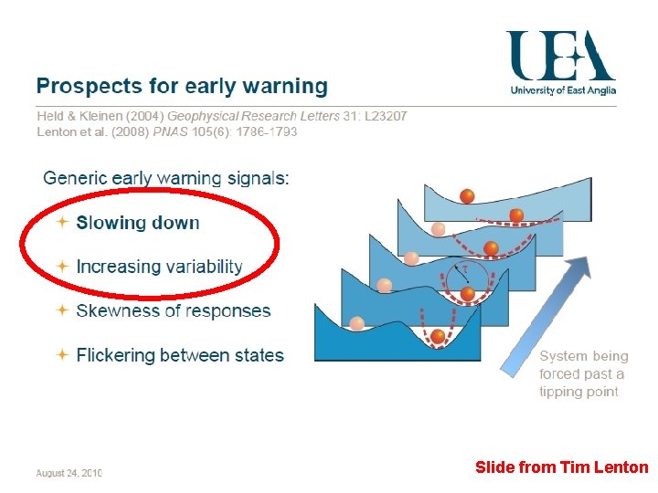
Slide from Tim Lenton

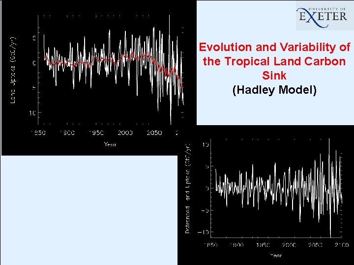
Evolution and Variability of the Tropical Land Carbon Sink (Hadley Model)

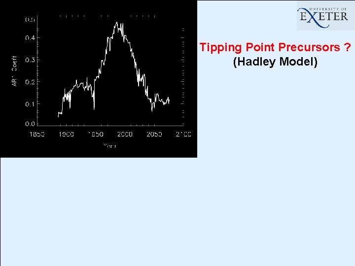
Tipping Point Precursors ? (Hadley Model)

Ongoing Work Ø Spatial correlation as a possible precursor of Amazon dieback (Huntingford, Lenton). Ø Test of “slowing down” as forewarning of Amazon dieback against an ensemble of climate-carbon cycle projections (Booth, Cox). Ø Development of simple models to demonstrate different types of tipping points and to investigate their precursors (Vitolo, Ashwin).

Any Questions ?