NATCOR Stochastic Modelling Course Inventory Control Part 1

NATCOR Stochastic Modelling Course Inventory Control – Part 1 Adam Letchford Department of Management Science Lancaster University Management School

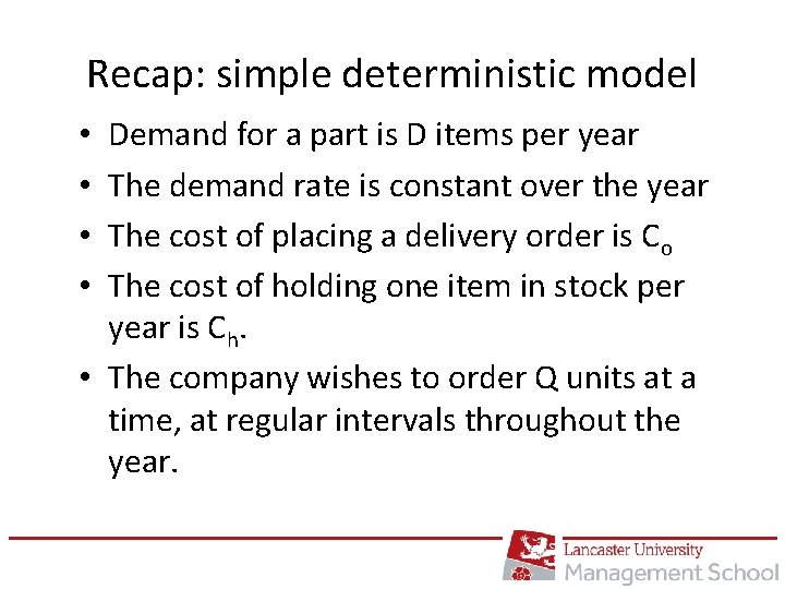
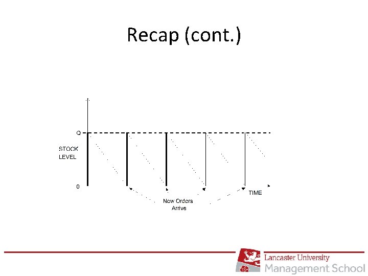
Recap: simple deterministic model Demand for a part is D items per year The demand rate is constant over the year The cost of placing a delivery order is Co The cost of holding one item in stock per year is Ch. • The company wishes to order Q units at a time, at regular intervals throughout the year. • •

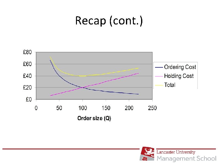
Recap (cont. )

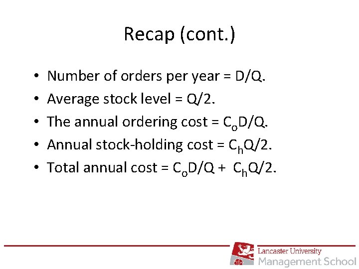
Recap (cont. ) • • • Number of orders per year = D/Q. Average stock level = Q/2. The annual ordering cost = Co. D/Q. Annual stock-holding cost = Ch. Q/2. Total annual cost = Co. D/Q + Ch. Q/2.

Recap (cont. )

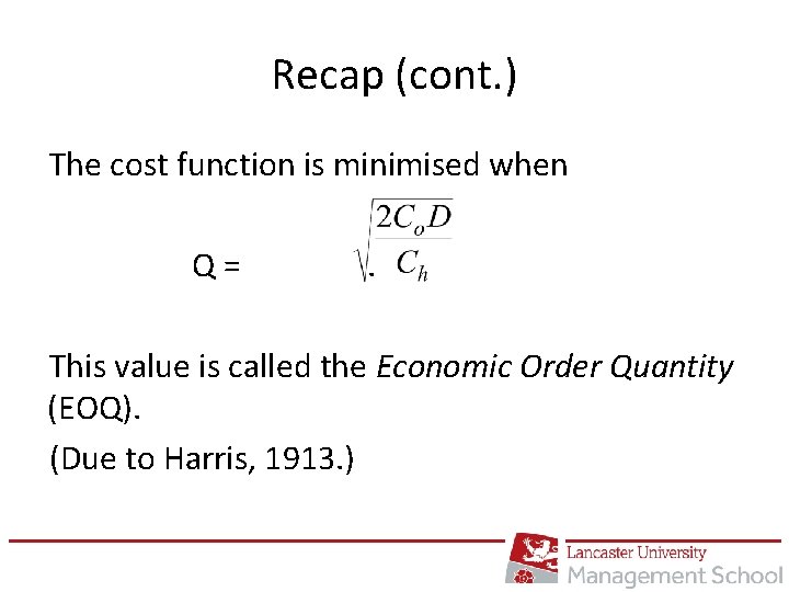
Recap (cont. ) The cost function is minimised when Q= . This value is called the Economic Order Quantity (EOQ). (Due to Harris, 1913. )

Stochastic Aspects In real life, there are two important things to take into account: 1. Lead Time (L): there is usually a delay between placing an order and the order arriving. 2. Stochastic demand: the demand per unit time usually is not constant, but varies according to a known distribution. 7

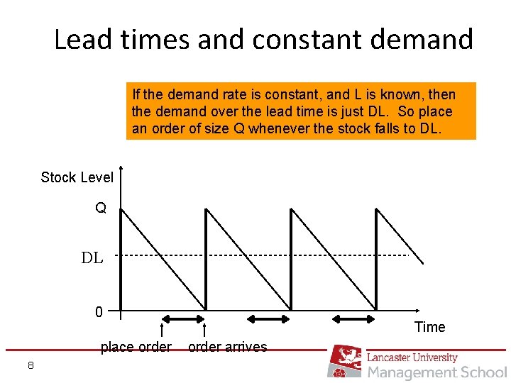
Lead times and constant demand If the demand rate is constant, and L is known, then the demand over the lead time is just DL. So place an order of size Q whenever the stock falls to DL. Stock Level Q DL 0 place order 8 Time order arrives

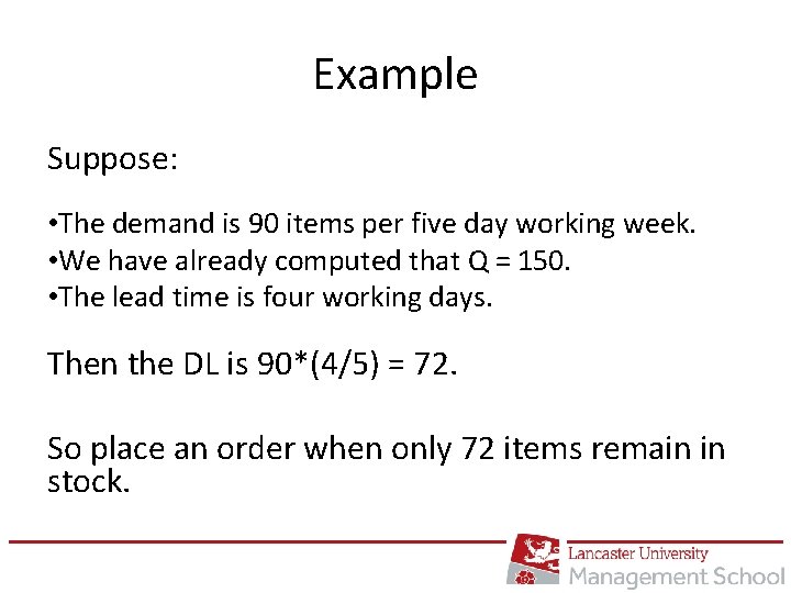
Example Suppose: • The demand is 90 items per five day working week. • We have already computed that Q = 150. • The lead time is four working days. Then the DL is 90*(4/5) = 72. So place an order when only 72 items remain in stock.

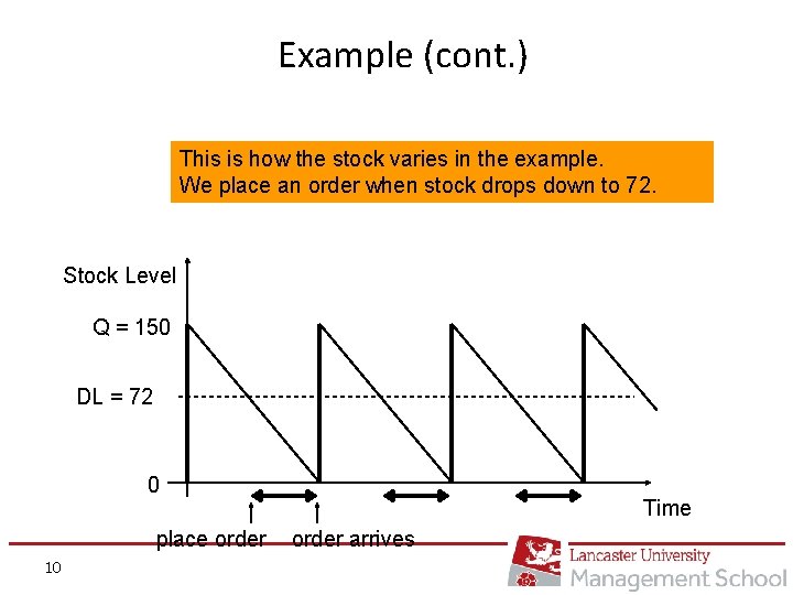
Example (cont. ) This is how the stock varies in the example. We place an order when stock drops down to 72. Stock Level Q = 150 DL = 72 0 place order 10 Time order arrives

Lead times and stochastic demand • Now suppose that demand is stochastic. • We assume that the demand per unit time period follows some known probability distribution. • For example, we may know that the demand in a five-day working week follows a normal distribution with a mean of 90 and a standard deviation of 25. 11

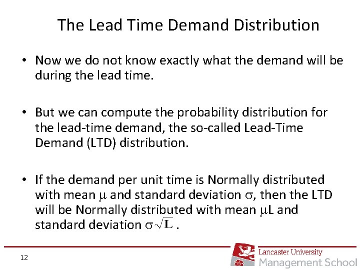
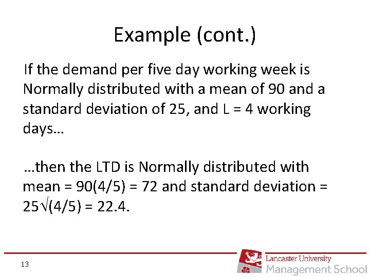
The Lead Time Demand Distribution • Now we do not know exactly what the demand will be during the lead time. • But we can compute the probability distribution for the lead-time demand, the so-called Lead-Time Demand (LTD) distribution. • If the demand per unit time is Normally distributed with mean and standard deviation , then the LTD will be Normally distributed with mean L and standard deviation . 12

Example (cont. ) If the demand per five day working week is Normally distributed with a mean of 90 and a standard deviation of 25, and L = 4 working days… …then the LTD is Normally distributed with mean = 90(4/5) = 72 and standard deviation = 25 (4/5) = 22. 4. 13

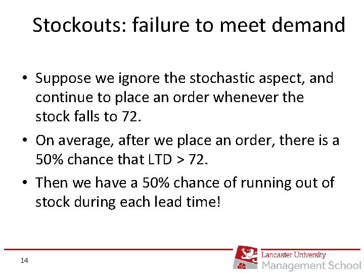
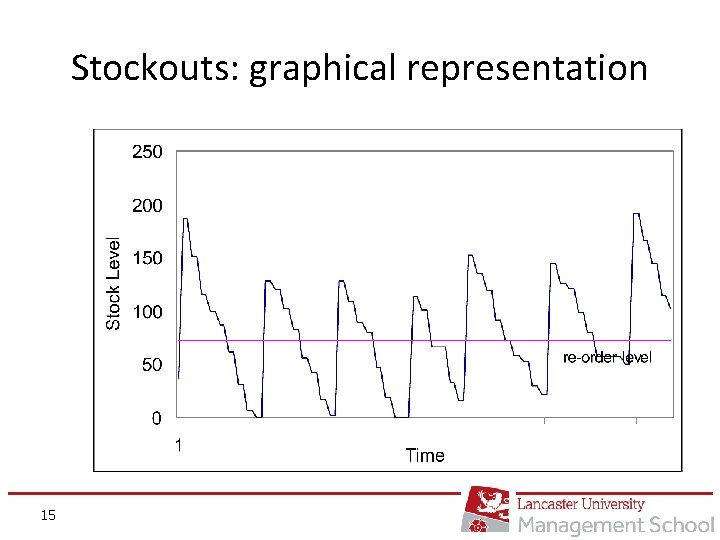
Stockouts: failure to meet demand • Suppose we ignore the stochastic aspect, and continue to place an order whenever the stock falls to 72. • On average, after we place an order, there is a 50% chance that LTD > 72. • Then we have a 50% chance of running out of stock during each lead time! 14

Stockouts: graphical representation 15

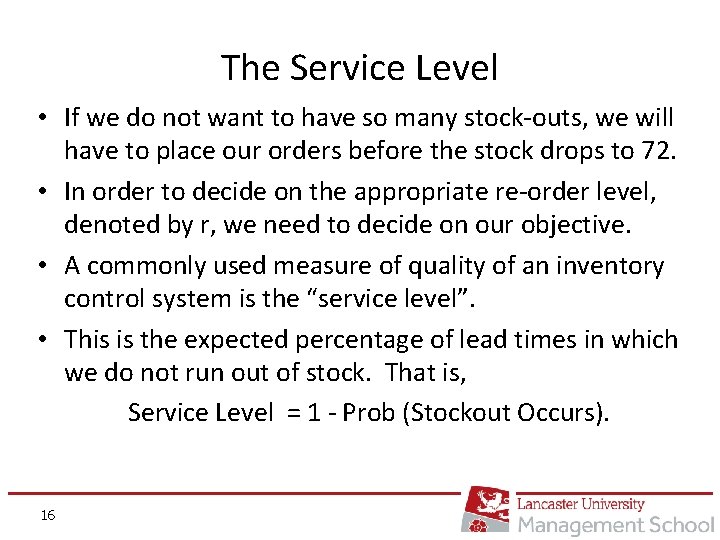
The Service Level • If we do not want to have so many stock-outs, we will have to place our orders before the stock drops to 72. • In order to decide on the appropriate re-order level, denoted by r, we need to decide on our objective. • A commonly used measure of quality of an inventory control system is the “service level”. • This is the expected percentage of lead times in which we do not run out of stock. That is, Service Level = 1 - Prob (Stockout Occurs). 16

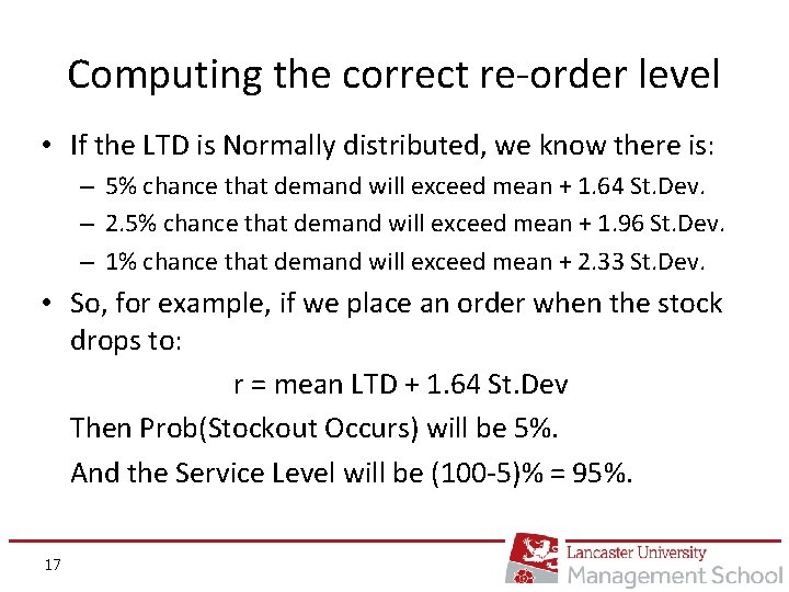
Computing the correct re-order level • If the LTD is Normally distributed, we know there is: – 5% chance that demand will exceed mean + 1. 64 St. Dev. – 2. 5% chance that demand will exceed mean + 1. 96 St. Dev. – 1% chance that demand will exceed mean + 2. 33 St. Dev. • So, for example, if we place an order when the stock drops to: r = mean LTD + 1. 64 St. Dev Then Prob(Stockout Occurs) will be 5%. And the Service Level will be (100 -5)% = 95%. 17

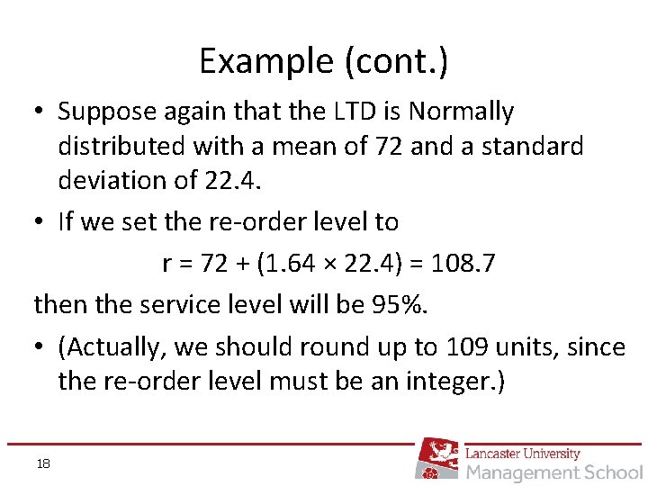
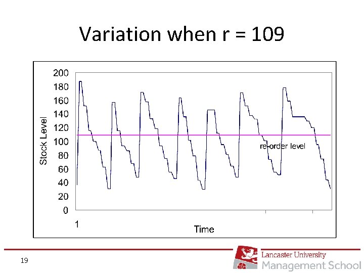
Example (cont. ) • Suppose again that the LTD is Normally distributed with a mean of 72 and a standard deviation of 22. 4. • If we set the re-order level to r = 72 + (1. 64 × 22. 4) = 108. 7 then the service level will be 95%. • (Actually, we should round up to 109 units, since the re-order level must be an integer. ) 18

Variation when r = 109 19

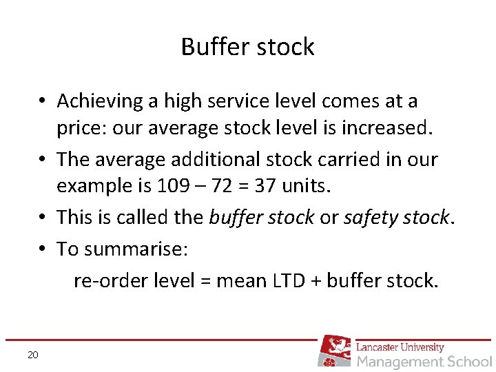
Buffer stock • Achieving a high service level comes at a price: our average stock level is increased. • The average additional stock carried in our example is 109 – 72 = 37 units. • This is called the buffer stock or safety stock. • To summarise: re-order level = mean LTD + buffer stock. 20

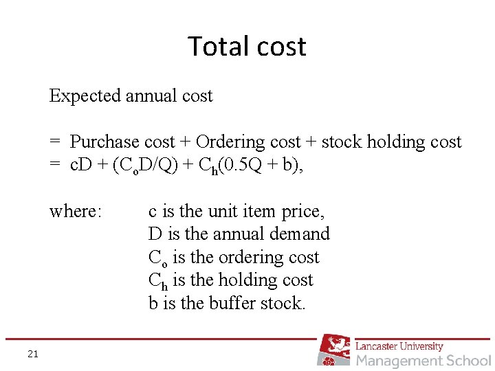
Total cost Expected annual cost = Purchase cost + Ordering cost + stock holding cost = c. D + (Co. D/Q) + Ch(0. 5 Q + b), where: 21 c is the unit item price, D is the annual demand Co is the ordering cost Ch is the holding cost b is the buffer stock.

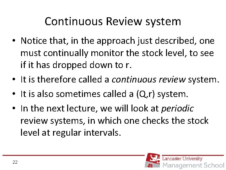
Continuous Review system • Notice that, in the approach just described, one must continually monitor the stock level, to see if it has dropped down to r. • It is therefore called a continuous review system. • It is also sometimes called a (Q, r) system. • In the next lecture, we will look at periodic review systems, in which one checks the stock level at regular intervals. 22