NATCOR Stochastic Modelling Course Inventory Control Part 3

NATCOR Stochastic Modelling Course Inventory Control – Part 3 Adam Letchford Department of Management Science Lancaster University Management School

Multi-Item Problems • So far, we have only considered problems in which there is a single product type (“item”) to order. • In real life we typically have many items to order. • This leads to some complications. • We now briefly consider three commonly-used multiitem models. • For simplicity we assume demand is deterministic. • We let n denote the number of items.

Variant I: Shared Space • Let item i have annual demand Di, order cost Co(i) and annual holding cost Ch(i). • We may also have lower bounds li and upper bounds ui for the delivery quantities. • Now suppose that one unit of item i takes up si space, and the total space available is S. • Each item must be ordered at regular intervals.

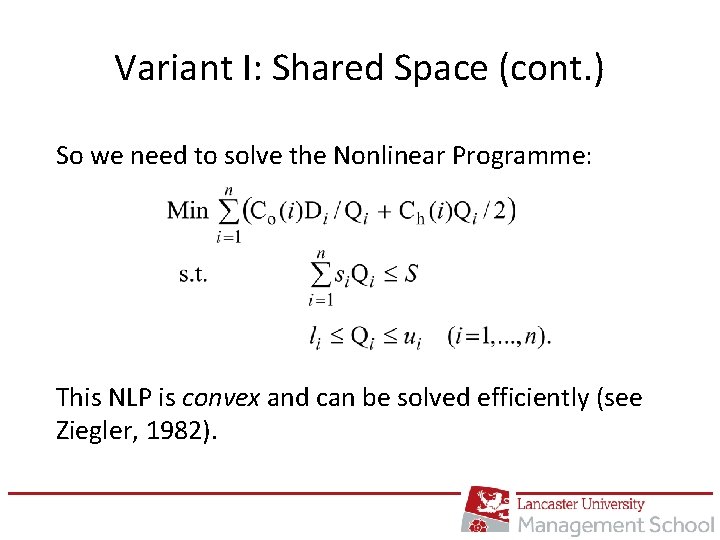
Variant I: Shared Space (cont. ) If order quantity for item i is Qi, then: • number of times i ordered per year is Di/Qi • annual ordering cost for i is Co(i) Di/Qi • average amount of i in stock is Qi/2 • annual cost of holding i in stock is Ch(i) Qi/2.

Variant I: Shared Space (cont. ) So we need to solve the Nonlinear Programme: This NLP is convex and can be solved efficiently (see Ziegler, 1982).

Variant II: Clustered Items • Now forget about the issue of shared space. • Suppose that the company wish to make inventory control easier by grouping the items into k “clusters”. • We are free to choose integers T 1, …, Tk so that items in cluster i are ordered every Ti time units. • E. g. , items in cluster 1 ordered every 4 weeks, items in cluster 2 ordered every 7 weeks, etc. • The optimal clustering can be computed efficiently, by dynamic programming (Chakaravarty, 1981).

Variant III: Joint Replenishment Now suppose that the n items all come from the same supplier. Then, if several different items are delivered at the same time, there may be a discount. One way to model the discount structure is to suppose that we have a “major” delivery cost M, together with a “minor” delivery cost mi for each item i. The cost of a delivery is then the major cost plus the sum of the relevant minor costs.

Variant III: Joint Replenishment (cont. ) • The resulting problem is called the Joint Replenishment Problem (JRP). • It can be formulated as a mixed-integer nonlinear programme. • It is “NP-hard”, which makes it unlikely that an efficient algorithm exists for all instances. • But some good heuristics exist. • See the survey Khouja & Goyal (2008).

And now for something completely different…

A “One-Off” Model: the Newsboy Problem • At the start of each day, a newsboy must decide on the number of papers to purchase. • Daily sales are stochastic, and are represented by the random variable x. • Purchasing one copy costs p. • Selling one copy yields revenue r (> p). • Scrapping an unsold copy costs s. • How many copies should he purchase?

Newsboy Problem (cont. ) It is helpful to compute: • Unit cost of over-stocking = co = p + s • Unit cost of under-stocking = cu = r – p. (Note: if desired, one can also attempt to incorporate “loss of customer goodwill” by increasing cu. )

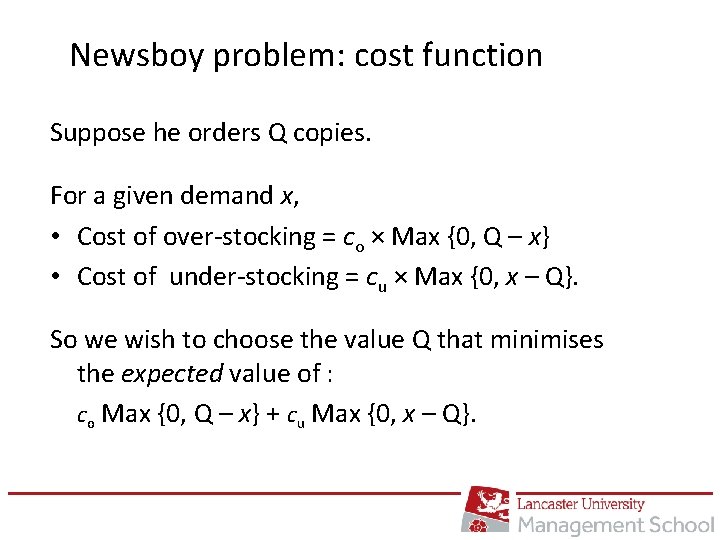
Newsboy problem: cost function Suppose he orders Q copies. For a given demand x, • Cost of over-stocking = co × Max {0, Q – x} • Cost of under-stocking = cu × Max {0, x – Q}. So we wish to choose the value Q that minimises the expected value of : co Max {0, Q – x} + cu Max {0, x – Q}.

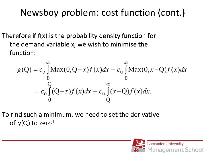
Newsboy problem: cost function (cont. ) Therefore if f(x) is the probability density function for the demand variable x, we wish to minimise the function: To find such a minimum, we need to set the derivative of g(Q) to zero!

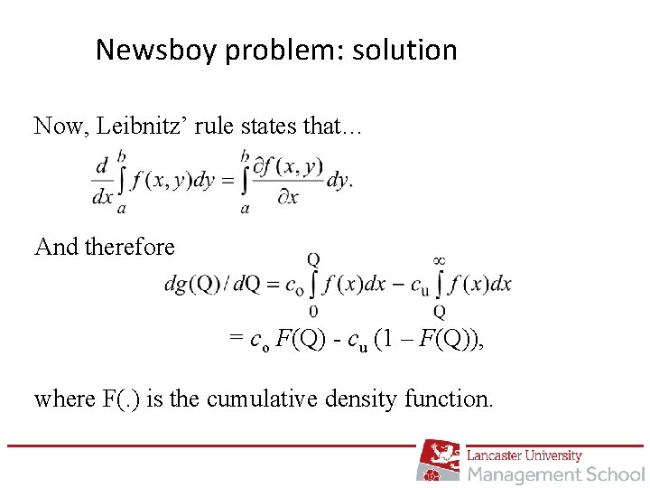
Newsboy problem: solution Now, Leibnitz’ rule states that… And therefore = co F(Q) - cu (1 – F(Q)), where F(. ) is the cumulative density function.

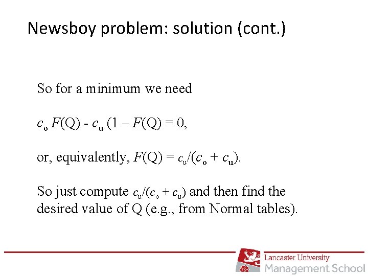
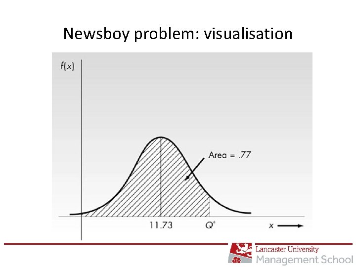
Newsboy problem: solution (cont. ) So for a minimum we need co F(Q) - cu (1 – F(Q) = 0, or, equivalently, F(Q) = cu/(co + cu). So just compute cu/(co + cu) and then find the desired value of Q (e. g. , from Normal tables).

Newsboy problem: visualisation

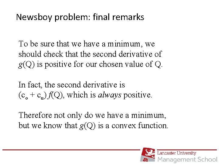
Newsboy problem: final remarks To be sure that we have a minimum, we should check that the second derivative of g(Q) is positive for our chosen value of Q. In fact, the second derivative is (co + cu) f(Q), which is always positive. Therefore not only do we have a minimum, but we know that g(Q) is a convex function.

References I: Books • W. J. Hopp & M. L. Spearman (2011) Factory Physics (3 rd edn. ) • S. Nahmias (2008) Production & Operations Analysis (6 th edn. ) • E. Porteus (2002) Foundations of Stochastic Inventory Theory. • E. A. Silver, D. F. Pyke & R. Peterson (1998) Inventory Management and Production Planning and Scheduling (3 rd edn. ) • D. Sipper & R. L. Bulfin Jr (1997) Production: Planning, Control and Integration.

References II: Papers • A. K. Chakaravarty (1981) Multi-item inventory aggregation into groups. J. Oper. Res. Soc. , 32, 19 -26. • F. W. Harris (1913) How many parts to make at once. Factory, The Magazine of Management, 10, 135 -136, 152. • M. Khouja & S. Goyal (2008) A review of the joint replenishment problem literature: 1989– 2005. Eur. J. Oper. Res. , 186, 1 -16. • H. Ziegler (1982) Solving certain singly constrained convex optimization problems in production planning. Oper. Res. Lett. , 1, 252– 256.