MTH 161 Introduction To Statistics Lecture 29 Dr

MTH 161: Introduction To Statistics Lecture 29 Dr. MUMTAZ AHMED

Review of Previous Lecture In last lecture we discussed: � Joint Distributions � Moment Generating Functions � Covariance � Related Examples 2

Objectives of Current Lecture In the current lecture: � Covariance: Some important Results � Describing Bivariate Data � Scatter Plot � Concept of Correlation � Properties of Correlation � Related examples and Excel Demo 3

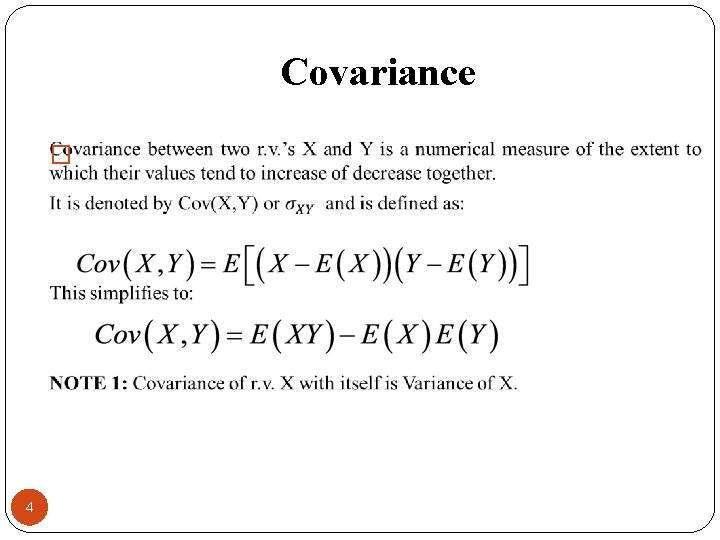
Covariance � 4

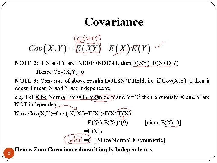
Covariance 5 NOTE 2: If X and Y are INDEPENDENT, then E(XY)=E(X) E(Y) Hence Cov(X, Y)=0 NOTE 3: Converse of above results DOESN’T Hold, i. e. if Cov(X, Y)=0 then it doesn’t mean X and Y are independent. e. g. Let X be Normal r. v with mean zero and Y=X 2 then obviously X and Y are NOT independent. Now Cov(X, Y)=Cov( X, X 2)=E(X 3)-E(X 2)E(X) =E(X 3)-E(X 2)*(0) [since E(X)=0] =E(X 3) =0 [Since Normal is symmetric] Hence, Zero Covariance doesn’t imply Independence.

Covariance Do Excel Demo 6

Describing Bivariate Data Sometimes, our interest lies in finding the “relationship”, or “association”, between two variables. This can be done by the following methods: � Scatter Plot � Correlation � Regression Analysis 7

Scatter Plot A first step in finding whether or not a relationship between two variables exists, is to plot each pair of independent-dependent observations {(Xi, Yi)}, i=1, 2, . . , n as a point on a graph paper. Such a diagram is called a Scatter Diagram or Scatter Plot. Usually, independent variable is taken along X-axis and dependent variable is taken along Y-axis. 8

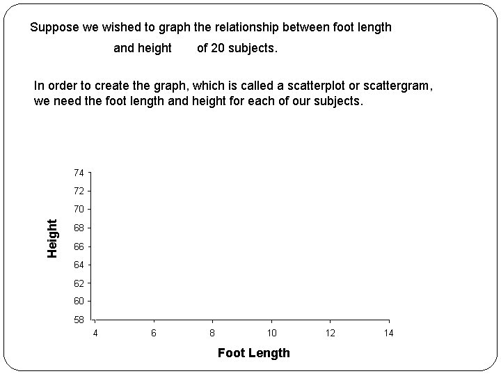
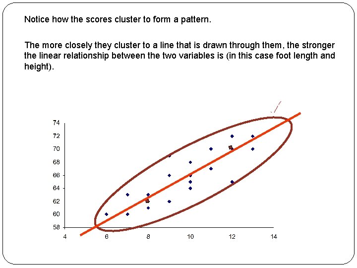
Suppose we wished to graph the relationship between foot length and height of 20 subjects. In order to create the graph, which is called a scatterplot or scattergram, we need the foot length and height for each of our subjects. 74 72 Height 70 68 66 64 62 60 58 4 6 8 10 Foot Length 12 14

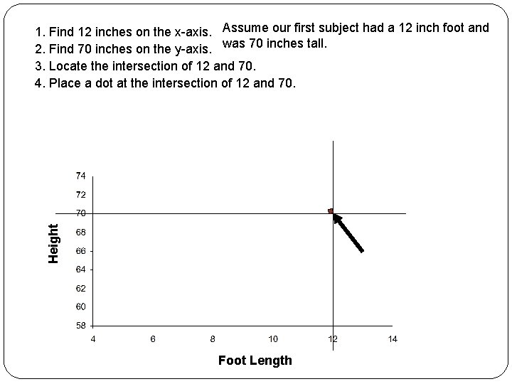
Height 1. Find 12 inches on the x-axis. Assume our first subject had a 12 inch foot and 2. Find 70 inches on the y-axis. was 70 inches tall. 3. Locate the intersection of 12 and 70. 4. Place a dot at the intersection of 12 and 70. Foot Length

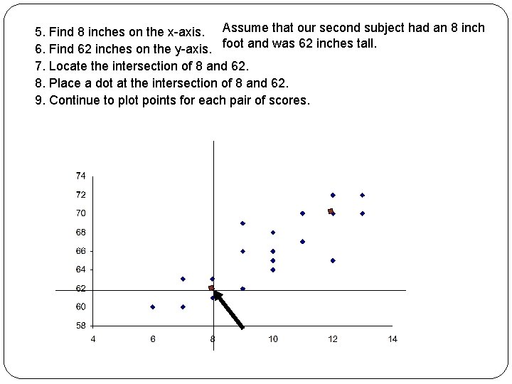
5. Find 8 inches on the x-axis. Assume that our second subject had an 8 inch 6. Find 62 inches on the y-axis. foot and was 62 inches tall. 7. Locate the intersection of 8 and 62. 8. Place a dot at the intersection of 8 and 62. 9. Continue to plot points for each pair of scores.

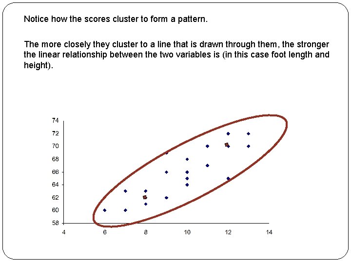
Notice how the scores cluster to form a pattern. The more closely they cluster to a line that is drawn through them, the stronger the linear relationship between the two variables is (in this case foot length and height).

Notice how the scores cluster to form a pattern. The more closely they cluster to a line that is drawn through them, the stronger the linear relationship between the two variables is (in this case foot length and height).

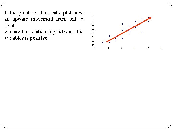
If the points on the scatterplot have an upward movement from left to right, we say the relationship between the variables is positive.

If the points on the scatterplot have an upward movement from left to right, we say the relationship between the variables is positive.

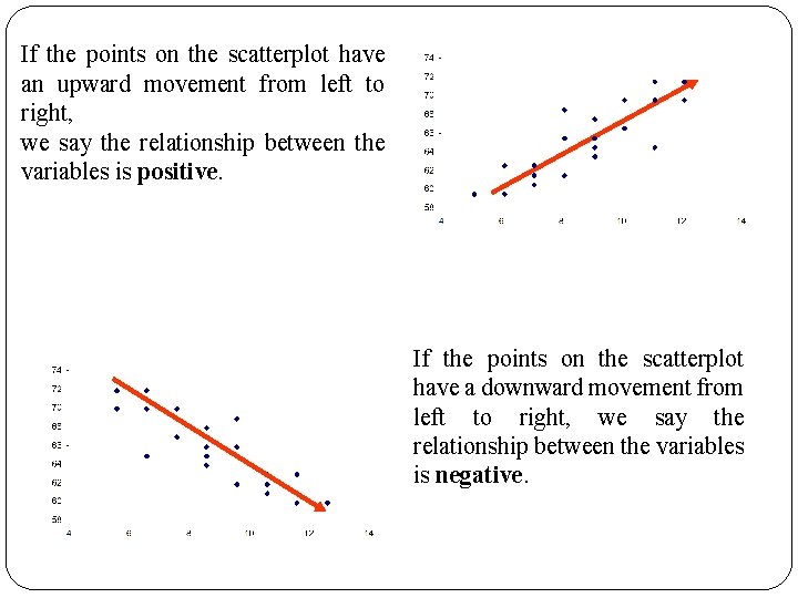
If the points on the scatterplot have an upward movement from left to right, we say the relationship between the variables is positive. If the points on the scatterplot have a downward movement from left to right, we say the relationship between the variables is negative.

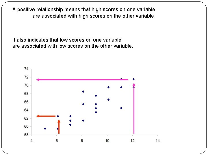
A positive relationship means that high scores on one variable are associated with high scores on the other variable It also indicates that low scores on one variable are associated with low scores on the other variable.

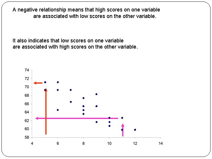
A negative relationship means that high scores on one variable are associated with low scores on the other variable. It also indicates that low scores on one variable are associated with high scores on the other variable.

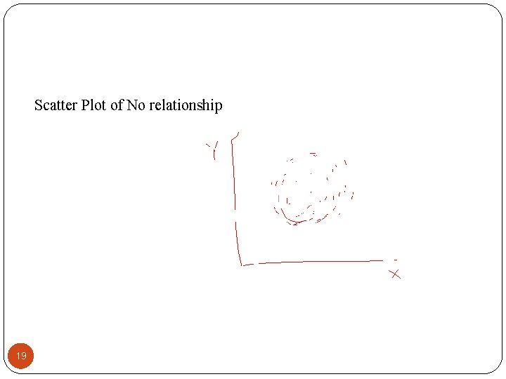
Scatter Plot of No relationship 19

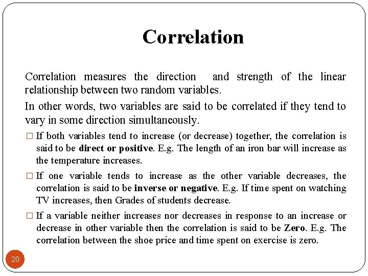
Correlation measures the direction and strength of the linear relationship between two random variables. In other words, two variables are said to be correlated if they tend to vary in some direction simultaneously. � If both variables tend to increase (or decrease) together, the correlation is said to be direct or positive. E. g. The length of an iron bar will increase as the temperature increases. � If one variable tends to increase as the other variable decreases, the correlation is said to be inverse or negative. E. g. If time spent on watching TV increases, then Grades of students decrease. � If a variable neither increases nor decreases in response to an increase or decrease in other variable then the correlation is said to be Zero. E. g. The correlation between the shoe price and time spent on exercise is zero. 20

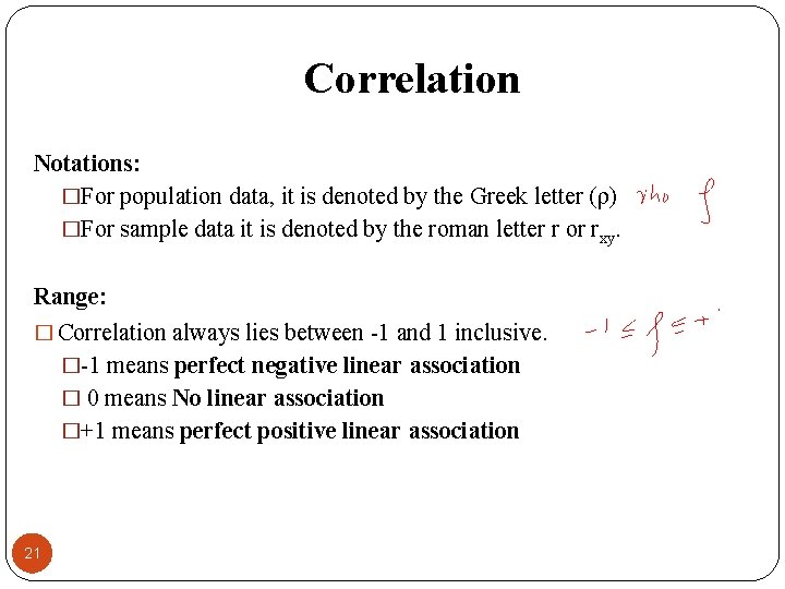
Correlation Notations: �For population data, it is denoted by the Greek letter (ρ) �For sample data it is denoted by the roman letter r or rxy. Range: � Correlation always lies between -1 and 1 inclusive. �-1 means perfect negative linear association � 0 means No linear association �+1 means perfect positive linear association 21

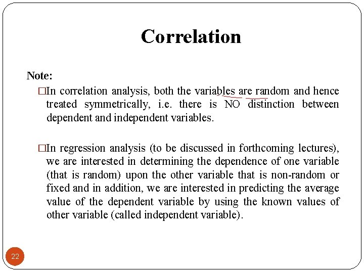
Correlation Note: �In correlation analysis, both the variables are random and hence treated symmetrically, i. e. there is NO distinction between dependent and independent variables. �In regression analysis (to be discussed in forthcoming lectures), we are interested in determining the dependence of one variable (that is random) upon the other variable that is non-random or fixed and in addition, we are interested in predicting the average value of the dependent variable by using the known values of other variable (called independent variable). 22

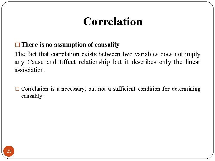
Correlation � There is no assumption of causality The fact that correlation exists between two variables does not imply any Cause and Effect relationship but it describes only the linear association. � Correlation is a necessary, but not a sufficient condition for determining causality. 23

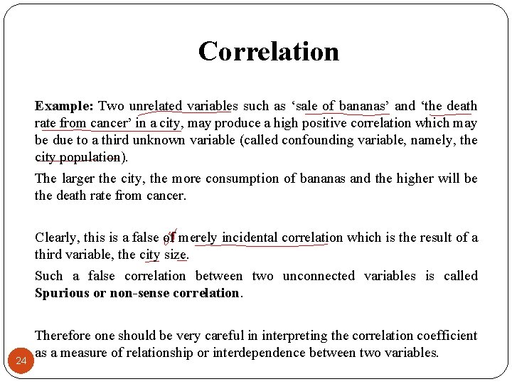
Correlation Example: Two unrelated variables such as ‘sale of bananas’ and ‘the death rate from cancer’ in a city, may produce a high positive correlation which may be due to a third unknown variable (called confounding variable, namely, the city population). The larger the city, the more consumption of bananas and the higher will be the death rate from cancer. Clearly, this is a false of merely incidental correlation which is the result of a third variable, the city size. Such a false correlation between two unconnected variables is called Spurious or non-sense correlation. 24 Therefore one should be very careful in interpreting the correlation coefficient as a measure of relationship or interdependence between two variables.

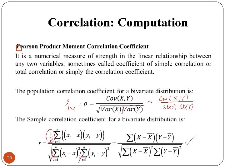
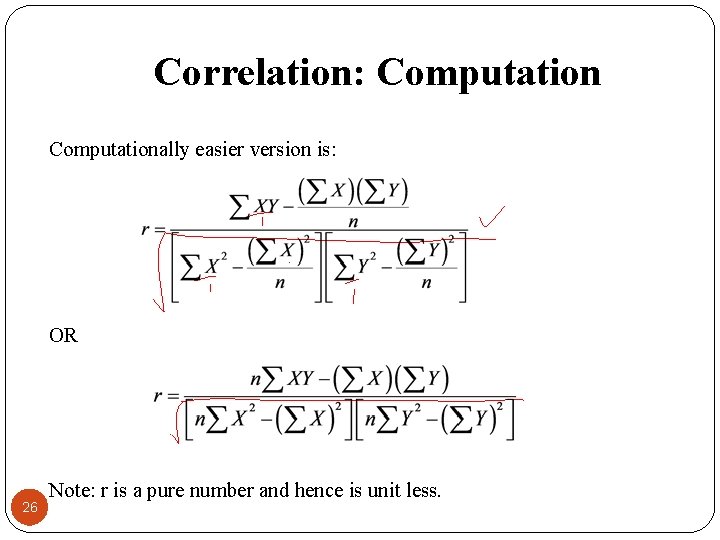
Correlation: Computation � 25

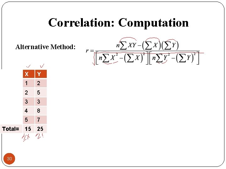
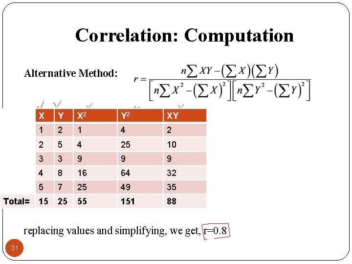
Correlation: Computationally easier version is: OR 26 Note: r is a pure number and hence is unit less.

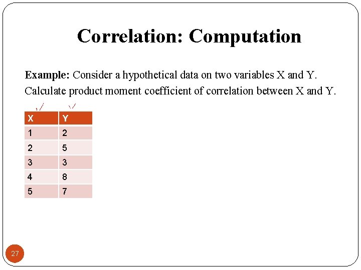
Correlation: Computation Example: Consider a hypothetical data on two variables X and Y. Calculate product moment coefficient of correlation between X and Y. 27 X Y 1 2 2 5 3 3 4 8 5 7

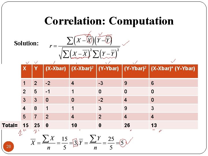
Correlation: Computation Solution: Total= 28 X Y (X-Xbar)2 (Y-Ybar)2 (X-Xbar)* (Y-Ybar) 1 2 -2 4 -3 9 6 2 5 -1 1 0 0 0 3 3 0 0 -2 4 0 4 8 1 1 3 9 3 5 7 2 4 4 15 25 0 10 0 26 13

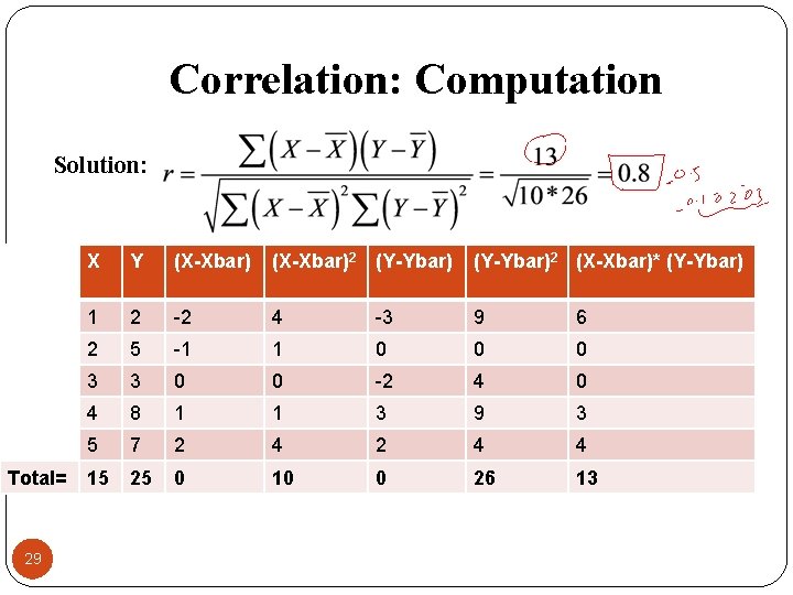
Correlation: Computation Solution: Total= 29 X Y (X-Xbar)2 (Y-Ybar)2 (X-Xbar)* (Y-Ybar) 1 2 -2 4 -3 9 6 2 5 -1 1 0 0 0 3 3 0 0 -2 4 0 4 8 1 1 3 9 3 5 7 2 4 4 15 25 0 10 0 26 13

Correlation: Computation Alternative Method: Total= 30 X Y 1 2 2 5 3 3 4 8 5 7 15 25

Correlation: Computation Alternative Method: Total= X Y X 2 Y 2 XY 1 2 1 4 2 2 5 4 25 10 3 3 9 9 9 4 8 16 64 32 5 7 25 49 35 15 25 55 151 88 replacing values and simplifying, we get, r=0. 8 31

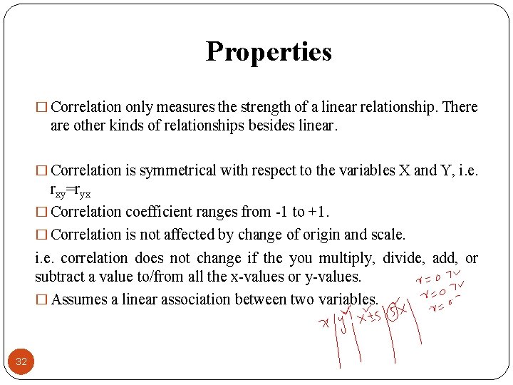
Properties � Correlation only measures the strength of a linear relationship. There are other kinds of relationships besides linear. � Correlation is symmetrical with respect to the variables X and Y, i. e. rxy=ryx � Correlation coefficient ranges from -1 to +1. � Correlation is not affected by change of origin and scale. i. e. correlation does not change if the you multiply, divide, add, or subtract a value to/from all the x-values or y-values. � Assumes a linear association between two variables. 32

Review Let’s review the main concepts: � Covariance: Some important Results � Describing Bivariate Data � Scatter Plot � Concept of Correlation � Properties of Correlation � Related examples and Excel Demo 33

Next Lecture In next lecture, we will study: � Common misconceptions about correlation � Related Examples 34