MTH 161 Introduction To Statistics Lecture 26 Dr

MTH 161: Introduction To Statistics Lecture 26 Dr. MUMTAZ AHMED

Review of Previous Lecture In last lecture we discussed: � Normal Distribution �Probability Density Function of Normal Distribution �Properties of Normal Distribution �Related examples 2

Objectives of Current Lecture In the current lecture: � Finding Area under the Normal Distribution � Normal Approximation to Binomial Distribution � Related examples 3

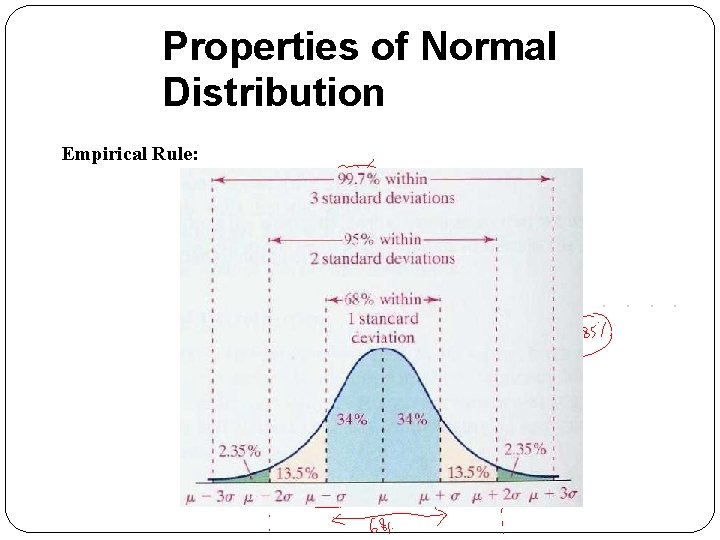
Properties of Normal Distribution Empirical Rule:

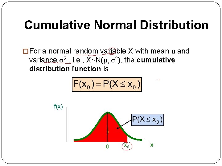
Cumulative Normal Distribution � For a normal random variable X with mean μ and variance σ2 , i. e. , X~N(μ, σ2), the cumulative distribution function is f(x) 0 x

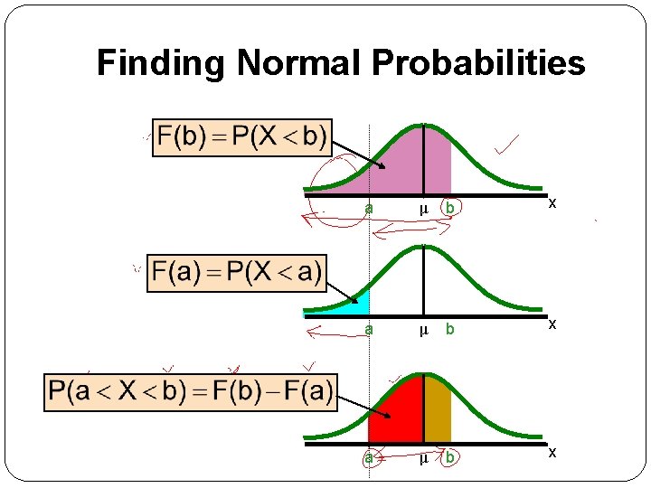
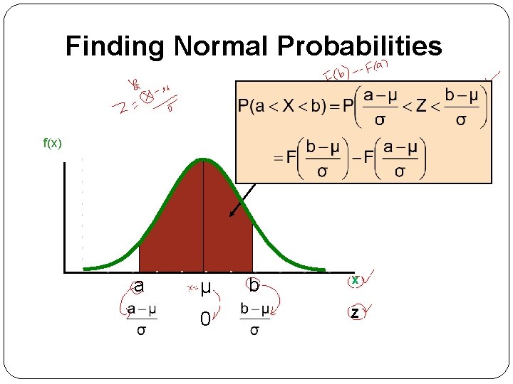
Finding Normal Probabilities a μ b x

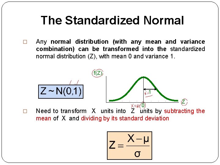
The Standardized Normal � Any normal distribution (with any mean and variance combination) can be transformed into the standardized normal distribution (Z), with mean 0 and variance 1. f(Z) 1 0 � Z Need to transform X units into Z units by subtracting the mean of X and dividing by its standard deviation

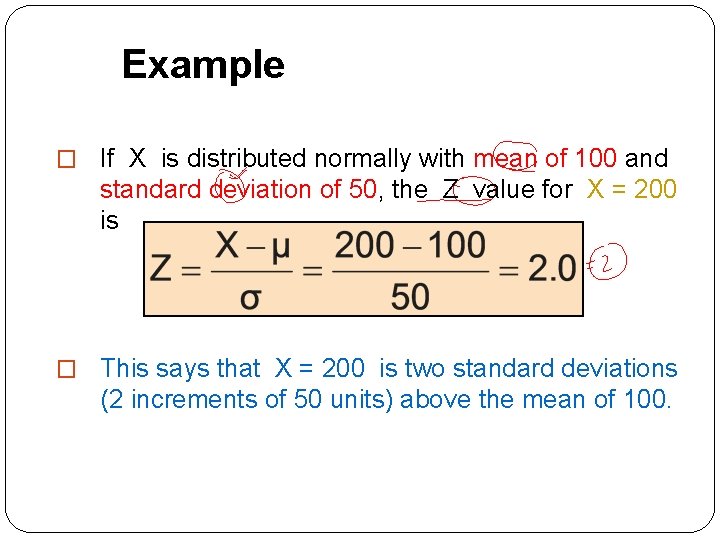
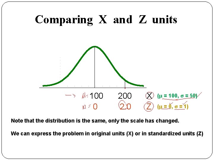
Example � If X is distributed normally with mean of 100 and standard deviation of 50, the Z value for X = 200 is � This says that X = 200 is two standard deviations (2 increments of 50 units) above the mean of 100.

Comparing X and Z units 100 0 200 2. 0 X Z (μ = 100, σ = 50) (μ = 0, σ = 1) Note that the distribution is the same, only the scale has changed. We can express the problem in original units (X) or in standardized units (Z)

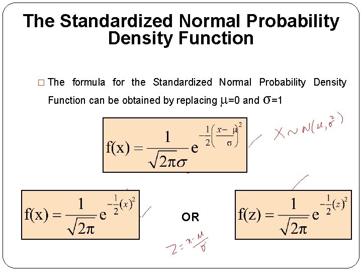
The Standardized Normal Probability Density Function � The formula for the Standardized Normal Probability Density Function can be obtained by replacing =0 and • OR σ=1

Finding Normal Probabilities f(x) a µ 0 b x Z

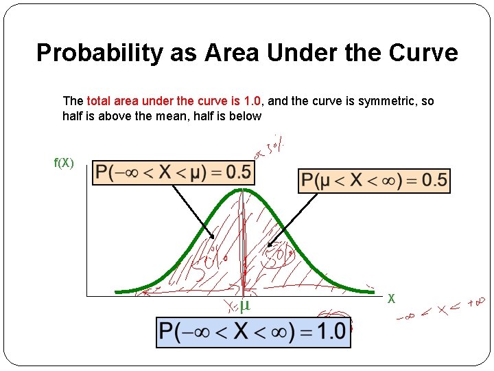
Probability as Area Under the Curve The total area under the curve is 1. 0, and the curve is symmetric, so half is above the mean, half is below f(X) 0. 5 μ X

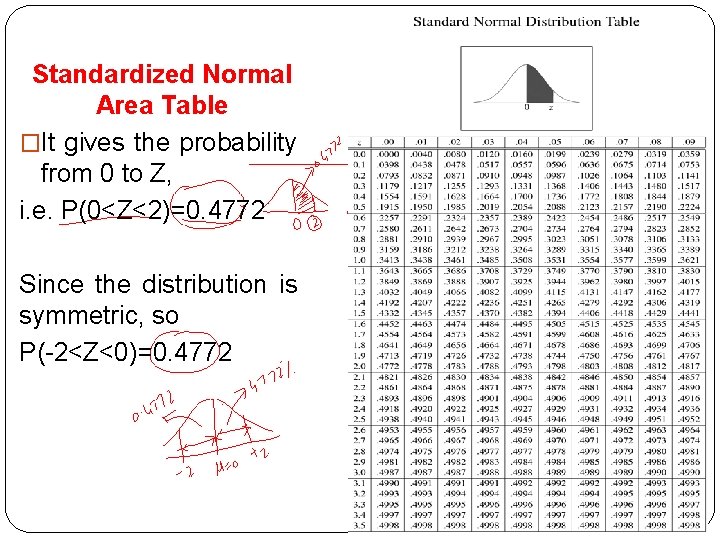
Standardized Normal Area Table �It gives the probability from 0 to Z, i. e. P(0<Z<2)=0. 4772 Since the distribution is symmetric, so P(-2<Z<0)=0. 4772

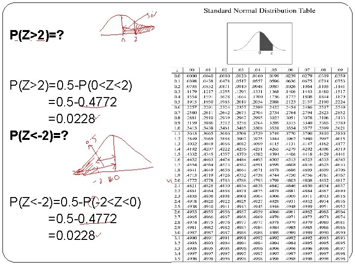
P(Z>2)=? P(Z>2)=0. 5 -P(0<Z<2) =0. 5 -0. 4772 =0. 0228 P(Z<-2)=? P(Z<-2)=0. 5 -P(-2<Z<0) =0. 5 -0. 4772 =0. 0228

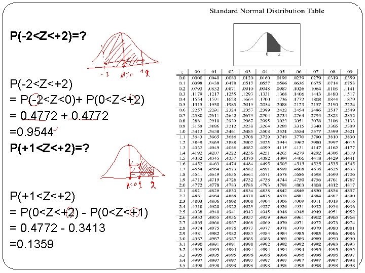
P(-2<Z<+2)=? P(-2<Z<+2) = P(-2<Z<0)+ P(0<Z<+2) = 0. 4772 + 0. 4772 =0. 9544 P(+1<Z<+2)=? P(+1<Z<+2) = P(0<Z<+2) - P(0<Z<+1) = 0. 4772 - 0. 3413 =0. 1359

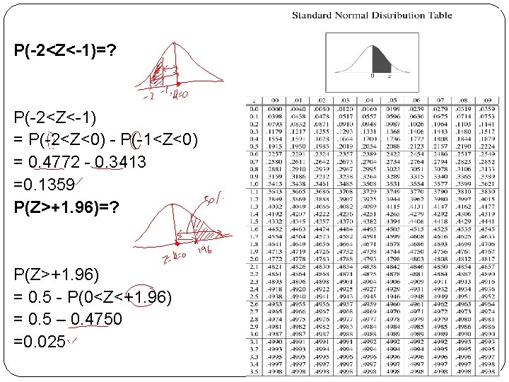
P(-2<Z<-1)=? P(-2<Z<-1) = P(-2<Z<0) - P(-1<Z<0) = 0. 4772 - 0. 3413 =0. 1359 P(Z>+1. 96)=? P(Z>+1. 96) = 0. 5 - P(0<Z<+1. 96) = 0. 5 – 0. 4750 =0. 025

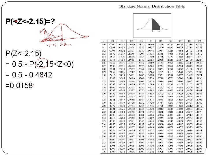
P(<Z<-2. 15)=? P(Z<-2. 15) = 0. 5 - P(-2. 15<Z<0) = 0. 5 - 0. 4842 =0. 0158

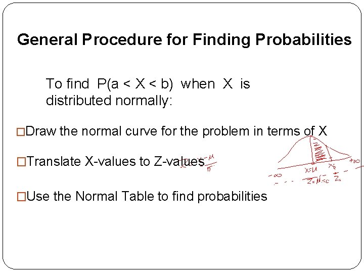
General Procedure for Finding Probabilities To find P(a < X < b) when X is distributed normally: �Draw the normal curve for the problem in terms of X �Translate X-values to Z-values �Use the Normal Table to find probabilities

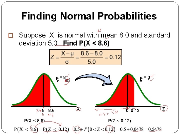
Finding Normal Probabilities � Suppose X is normal with mean 8. 0 and standard deviation 5. 0. Find P(X < 8. 6) μ=8 σ = 10 8 8. 6 P(X < 8. 6) μ=0 σ=1 X 0 0. 12 P(Z < 0. 12) Z

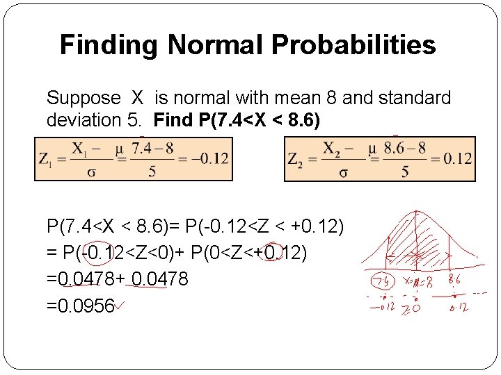
Finding Normal Probabilities Suppose X is normal with mean 8 and standard deviation 5. Find P(7. 4<X < 8. 6)= P(-0. 12<Z < +0. 12) = P(-0. 12<Z<0)+ P(0<Z<+0. 12) =0. 0478+ 0. 0478 =0. 0956

Review Let’s review the main concepts: � Cumulative Distribution Function � Finding Area under the Normal Distribution � Related examples 21

Next Lecture In next lecture, we will study: � Finding area under normal curve using MS-Excel � Normal Approximation to Binomial Distribution � Related Examples 22