MTH 161 Introduction To Statistics Lecture 15 Dr

MTH 161: Introduction To Statistics Lecture 15 Dr. MUMTAZ AHMED

Review of Previous Lecture In last lecture we discussed: Measures of Dispersion Variance and Standard Deviation Coefficient of Variation Properties of variance and standard deviation 2

Objectives of Current Lecture In the current lecture: Moments about Mean (Central Moments) Moments about any arbitrary Origin Moments about Zero Related Excel Demos 3

Objectives of Current Lecture In the current lecture: Relation b/w central moments and moments about origin Moment Ratios Skewness Kurtosis 4

Moments A moment is a quantitative measure of the shape of a set of points. The first moment is called the mean which describes the center of the distribution. The second moment is the variance which describes the spread of the observations around the center. Other moments describe other aspects of a distribution such as how the distribution is skewed from its mean or peaked. A moment designates the power to which deviations are raised before averaging them. 5

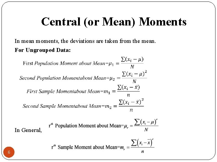
Central (or Mean) Moments In mean moments, the deviations are taken from the mean. For Ungrouped Data: In General, 6

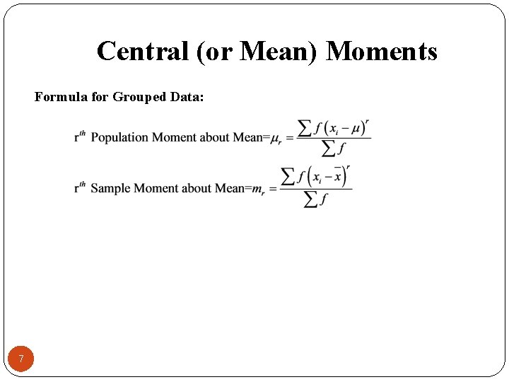
Central (or Mean) Moments Formula for Grouped Data: 7

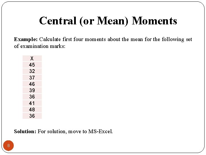
Central (or Mean) Moments Example: Calculate first four moments about the mean for the following set of examination marks: X 45 32 37 46 39 36 41 48 36 Solution: For solution, move to MS-Excel. 8

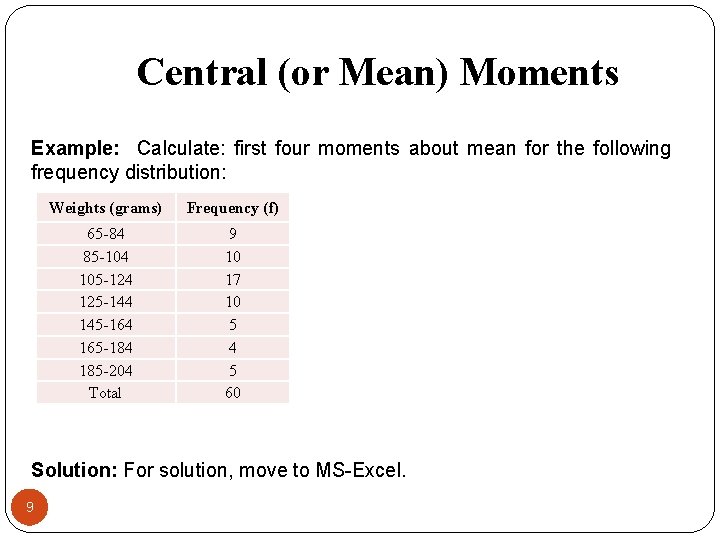
Central (or Mean) Moments Example: Calculate: first four moments about mean for the following frequency distribution: Weights (grams) Frequency (f) 65 -84 85 -104 105 -124 125 -144 145 -164 165 -184 185 -204 Total 9 10 17 10 5 4 5 60 Solution: For solution, move to MS-Excel. 9

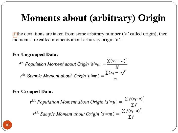
Moments about (arbitrary) Origin � 10

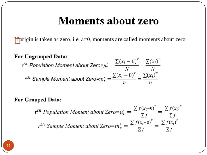
Moments about zero � 11

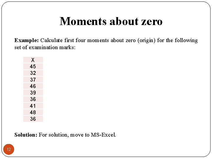
Moments about zero Example: Calculate first four moments about zero (origin) for the following set of examination marks: X 45 32 37 46 39 36 41 48 36 Solution: For solution, move to MS-Excel. 12

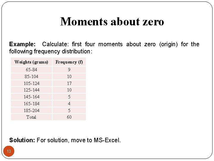
Moments about zero Example: Calculate: first four moments about zero (origin) for the following frequency distribution: Weights (grams) Frequency (f) 65 -84 85 -104 105 -124 125 -144 145 -164 165 -184 185 -204 Total 9 10 17 10 5 4 5 60 Solution: For solution, move to MS-Excel. 13

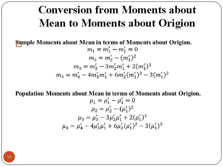
Conversion from Moments about Mean to Moments about Origion � 14

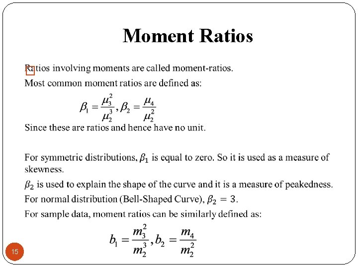
Moment Ratios � 15

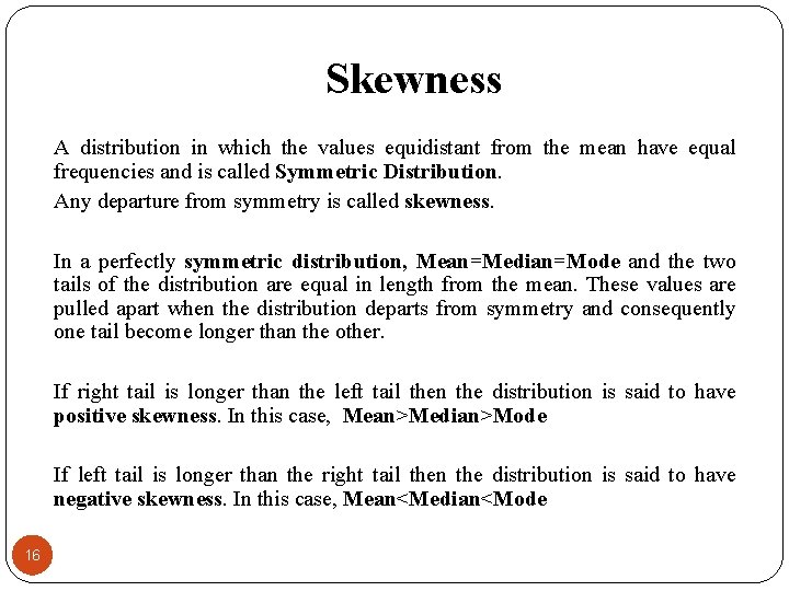
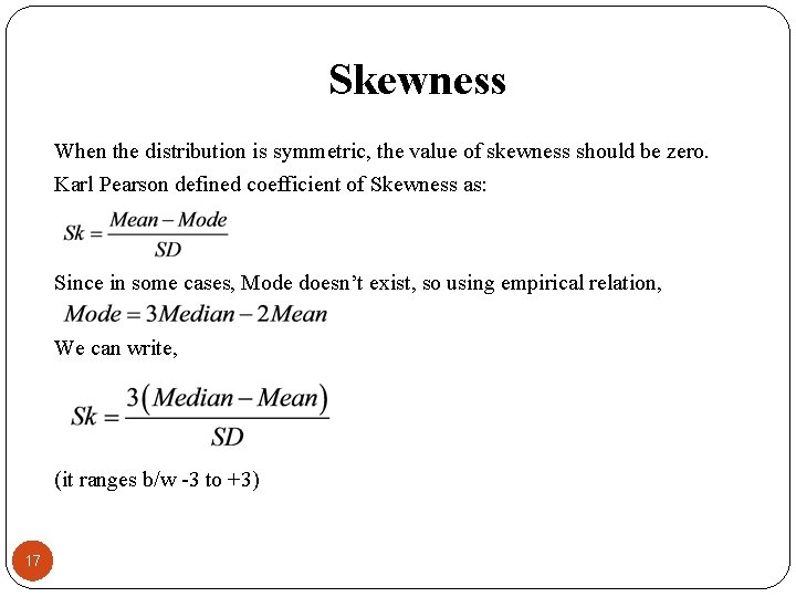
Skewness A distribution in which the values equidistant from the mean have equal frequencies and is called Symmetric Distribution. Any departure from symmetry is called skewness. In a perfectly symmetric distribution, Mean=Median=Mode and the two tails of the distribution are equal in length from the mean. These values are pulled apart when the distribution departs from symmetry and consequently one tail become longer than the other. If right tail is longer than the left tail then the distribution is said to have positive skewness. In this case, Mean>Median>Mode If left tail is longer than the right tail then the distribution is said to have negative skewness. In this case, Mean<Median<Mode 16

Skewness When the distribution is symmetric, the value of skewness should be zero. Karl Pearson defined coefficient of Skewness as: Since in some cases, Mode doesn’t exist, so using empirical relation, We can write, (it ranges b/w -3 to +3) 17

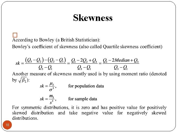
Skewness � 18

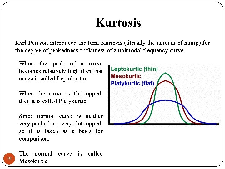
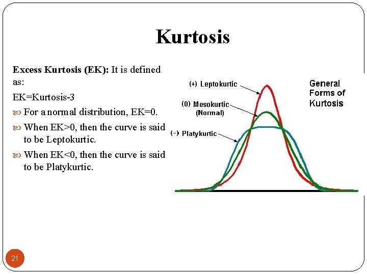
Kurtosis Karl Pearson introduced the term Kurtosis (literally the amount of hump) for the degree of peakedness or flatness of a unimodal frequency curve. When the peak of a curve becomes relatively high then that curve is called Leptokurtic. When the curve is flat-topped, then it is called Platykurtic. Since normal curve is neither very peaked nor very flat topped, so it is taken as a basis for comparison. 19 The normal curve is called Mesokurtic.

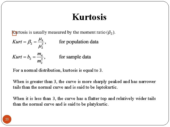
Kurtosis � For a normal distribution, kurtosis is equal to 3. When is greater than 3, the curve is more sharply peaked and has narrower tails than the normal curve and is said to be leptokurtic. When it is less than 3, the curve has a flatter top and relatively wider tails than the normal curve and is said to be platykurtic. 20

Kurtosis Excess Kurtosis (EK): It is defined as: EK=Kurtosis-3 For a normal distribution, EK=0. When EK>0, then the curve is said to be Leptokurtic. When EK<0, then the curve is said to be Platykurtic. 21

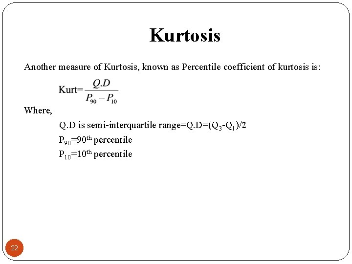
Kurtosis Another measure of Kurtosis, known as Percentile coefficient of kurtosis is: Where, Q. D is semi-interquartile range=Q. D=(Q 3 -Q 1)/2 P 90=90 th percentile P 10=10 th percentile 22

Describing a Frequency Distribution To describe the major characteristics of a frequency distribution, we need to calculate the following five quantities: The total number of observations in the data. A measure of central tendency (e. g. mean, median etc. ) that provides the information about the center or average value. A measure of dispersion (e. g. variance, SD etc. ) that indicates the spread of the data. A measure of skewness that shows lack of symmetry in frequency distribution. A measure of kurtosis that gives information about its peakedness. 23

Describing a Frequency Distribution It is interesting to note that all these quantities can be derived from the first four moments. For example, The first moment about zero is the arithmetic mean The second moment about mean is the variance. The third standardized moment is a measure of skewness. The fourth standardized moment is used to measure kurtosis. Thus first four moments play a key role in describing frequency distributions. 24

Review Let’s review the main concepts: Moments about Mean (Central Moments) Moments about any arbitrary Origin Moments about Zero Related Excel Demos 25

Review Let’s review the main concepts: Relation b/w central moments and moments about origin Moment Ratios Skewness Kurtosis 26

Next Lecture In next lecture, we will study: Introduction to Probability Definition and Basic concepts of probability 27