Modeling of discrete choice n alternative Individual enumerates


 Logit Model 選択肢が2つの場合 2項ロジットモデル When they have two alternatives n n 選択肢が多数(n個)ある場合")
")


を用いた ロジットモデルの推定 表 3. 15 バスの所要時間 表 3. 17 バスの所要費用 tBij c. Bij 1 2 3")

")


![Rにおける 尤度関数の定義と最大化 #対数尤度関数の定義 係数ベクトルxの関数と見なす. LL <- function (x){ vbus <- x[1] * tb + x[2]](https://slidetodoc.com/presentation_image_h/dd48bd9139eb7be45962be23df1bc9da/image-27.jpg "Rにおける 尤度関数の定義と最大化 #対数尤度関数の定義 係数ベクトルxの関数と見なす. LL <- function (x){ vbus <- x[1] * tb + x[2]")
![Rによる推定結果の表示 > res $par [1] -0. 081037584 -0. 004007811 0. 369193890 $value [1] -5.](https://slidetodoc.com/presentation_image_h/dd48bd9139eb7be45962be23df1bc9da/image-28.jpg "Rによる推定結果の表示 > res $par [1] -0. 081037584 -0. 004007811 0. 369193890 $value [1] -5.")
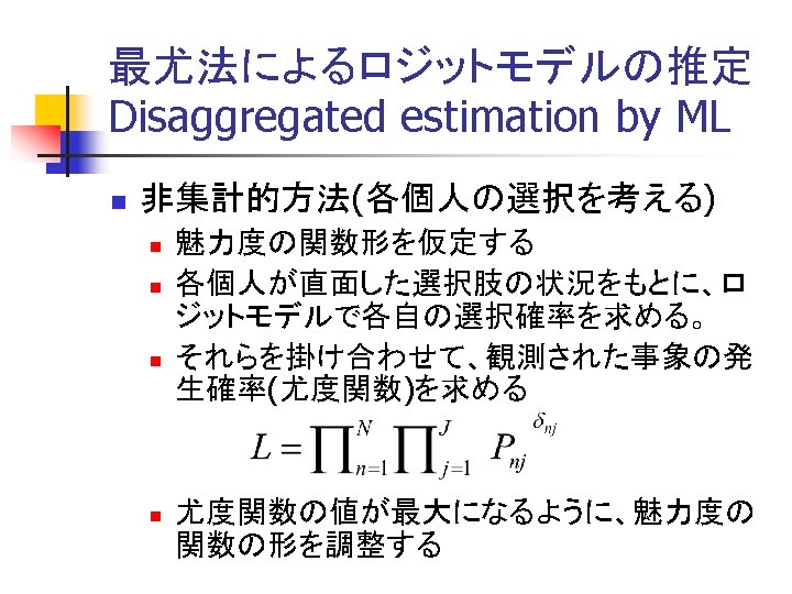
の時 Pure disaggregate data (one line for")
 ans 2 <- glm(pc ~ tsa+csa, family=quasibinomial(link=\"logit\")) summary(ans 2) Call: glm(formula")
 nc")
) summary(ans 3) Call:")


ehime. csv SEQ, 選択, 年齢, 保有台数, 鉄道可能性, 時間, 費用, バス可能性, 時間, 費用, 4輪可能性,")
 ### Multi Nomial Logit (MNL) estimation program (Original code by EHIME University)")

 Multinomial Logit Model install. packages(\"mlogit\") library(\"mlogit\") Dehime<-read. csv(\"ehime. csv\", header=T) Ehime <-mlogit. data(Dehime,")
 Multinomial Logit Model Call: mlogit(formula = Choice ~ time + cost - 1,")
 Multinomial Logit Model Call: mlogit(formula = Choice ~ time + cost, data =")

 ### Nested Logit estimation program (Original code by EHIME University) ###データファイルの読み込み Data<-read.")
- Slides: 58
離散的選択のモデル化 Modeling of discrete choice n 個人は,採りうる選択肢alternativeを列挙する Individual enumerates alternatives n 各選択肢の特徴と費用を考え、評価点をつける Assign evaluation points for each alternative. n 評価点が高いものを選ぶ Chose the alternative having the highest point China 60点 France 40点 USA 50点
確率的選択:評価点の差と選択率 Probablistic Choice n 実際には In many cases, n n 評価点に差が小さければ、どちらの選択肢も選ばれる可 能性がある Both alternatives are possibly chosen, if the difference of utility was not large. 評価点の差が大きいときは,片方しか選ばれない. 選択肢Aが選ばれる可能性 Probability of choice of A 1 Aが圧倒的に劣る Aが選ばれることはほとんどない Utility of A is very inferior to that of B, A is rarely chosen. 2つは同じ魅力 50%ずつ 0 Aが圧倒的に良い ほと んどAだけが選ばれる Utility of A is very superior to that of B, A is almost chosen. 選択肢Aの得点-選択肢Bの得点 Utility of A – Utility of B
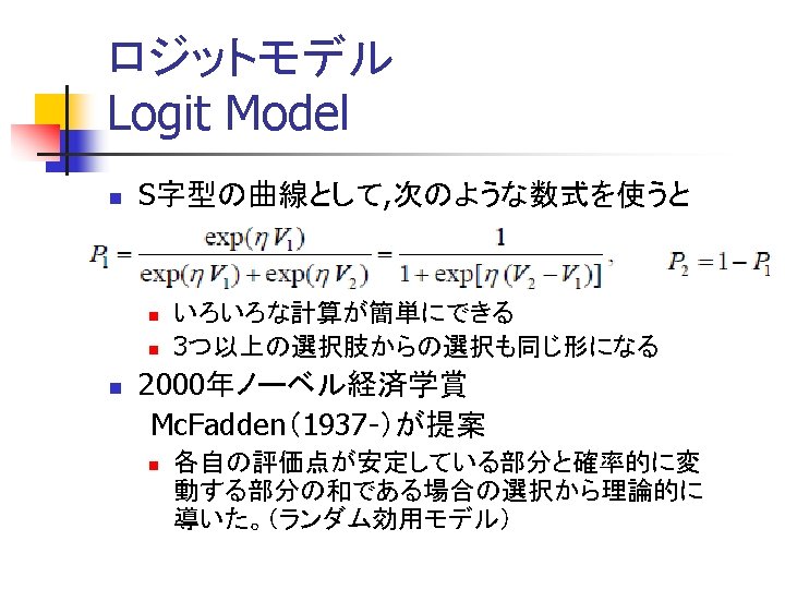
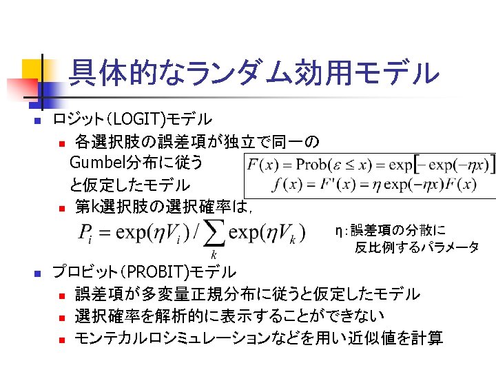
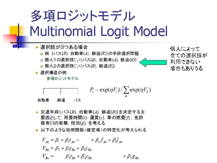
2項ロジットモデル Binary (Binomial) Logit Model 選択肢が2つの場合 2項ロジットモデル When they have two alternatives n n 選択肢が多数(n個)ある場合 Many alternatives 多項ロジットモデル Multinomial Logit
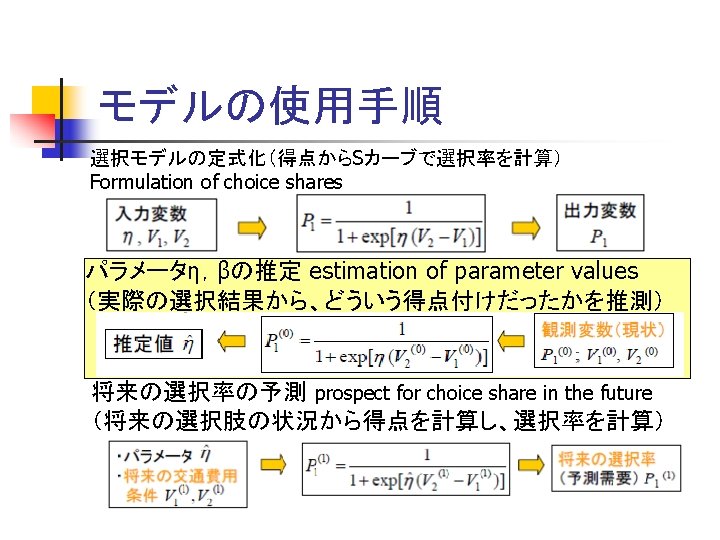
比率によるロジットモデルの推定 Estimation of parameters in Logit model based on the aggregated shares n 集計的方法(集団の選択率にあわせる) ある選択肢の状況下で観測された集団の選択確率p を用いる Observed share n ロジットモデルから、その時の 2つの選択肢の魅力度 VAとVBの差が逆算できる Utility differences are reversely calculated to meet with the obsereved share of two alternatives. n 魅力度の差がうまく一致するように、魅力度の関数の 形を調整する Adjust the parameters (functions) such that the proper utility difference are obtained. n
2項ロジットモデルの図解 Scheme of binary logit model V* 1 V 0 X 2 X 1
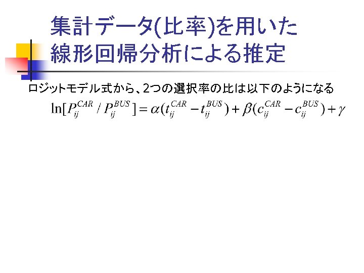
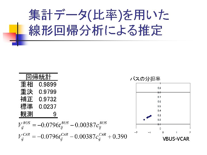
集計データ(比率)を用いた ロジットモデルの推定 表 3. 15 バスの所要時間 表 3. 17 バスの所要費用 tBij c. Bij 1 2 3 1 5 11 13 2 10 12 3 14 16 表 3. 19 バスの分担率 1 2 3 1 130 140 180 12 2 140 130 7 3 180 220 PBij 1 2 3 1 0. 273 0. 265 0. 253 220 2 0. 282 0. 248 0. 255 130 3 0. 239 0. 192 0. 244 単位:分 単位:円 表 3. 16 自動車の所要時 間 表 3. 18 自動車の所要費用 表 3. 20 自動車の分担率 c. Cij PCij t. Cij 1 2 3 1 21 45 58 1 0. 727 0. 735 0. 747 1 3 8 10 2 45 42 60 2 0. 718 0. 752 0. 745 2 8 7 11 3 58 60 19 3 0. 761 0. 808 0. 756 3 10 11 3 単位:分 単位:円
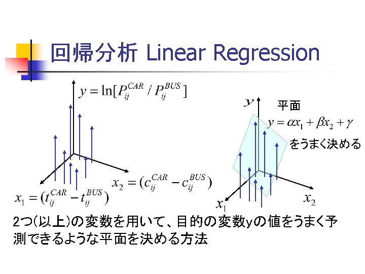
Rによる線形回帰 Linear regression by R tb <- c(5, 10, 14, 11, 12, 16, 13, 12, 7) tc <- c(3, 8, 10, 8, 7, 11, 10, 11, 3) cb <- c(130, 140, 180, 140, 130, 220, 180, 220, 130) cc <- c(21, 45, 58, 45, 42, 60, 58, 60, 19) pb <- c(0. 273, 0. 282, 0. 239, 0. 265, 0. 248, 0. 192, 0. 253, 0. 255, 0. 244) pc <- rep(1, 9)-pb lnpbpc <- log(pc/pb) tsa <- tc-tb csa <- cc-cb ans <- lm(lnpbpc ~ tsa+csa) summary(ans)
Rによる線形回帰の推定結果 Result of linear regression Call: lm(formula = lnpbpc ~ tsa + csa) Residuals: Min 1 Q Median 3 Q Max -0. 021913 -0. 017819 -0. 006659 0. 018098 0. 030403 Coefficients: Estimate Std. Error t value Pr(>|t|) (Intercept) 0. 3898049 0. 0446483 8. 731 0. 000125 *** tsa -0. 0795878 0. 0060416 -13. 173 1. 18 e-05 *** csa -0. 0038682 0. 0003171 -12. 200 1. 85 e-05 *** --Signif. codes: 0 ‘***’ 0. 001 ‘**’ 0. 01 ‘*’ 0. 05 ‘. ’ 0. 1 ‘ ’ 1 Residual standard error: 0. 0237 on 6 degrees of freedom Multiple R-squared: 0. 9799, Adjusted R-squared: 0. 9732 F-statistic: 146 on 2 and 6 DF, p-value: 8. 165 e-06
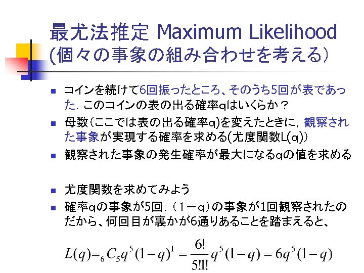
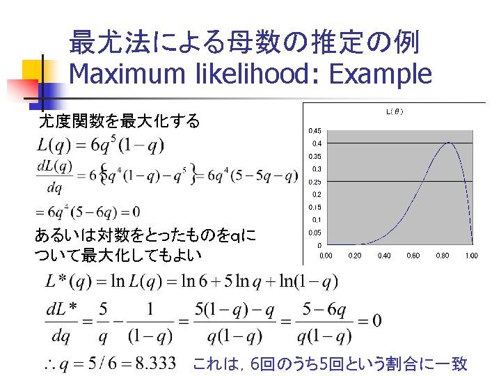
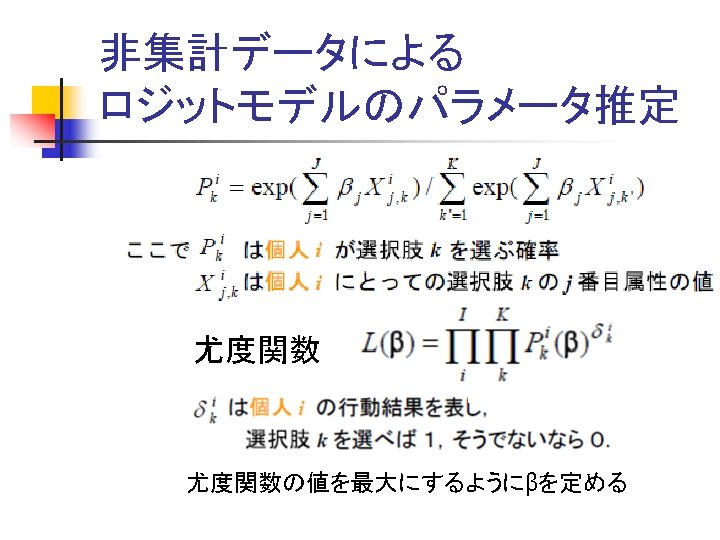
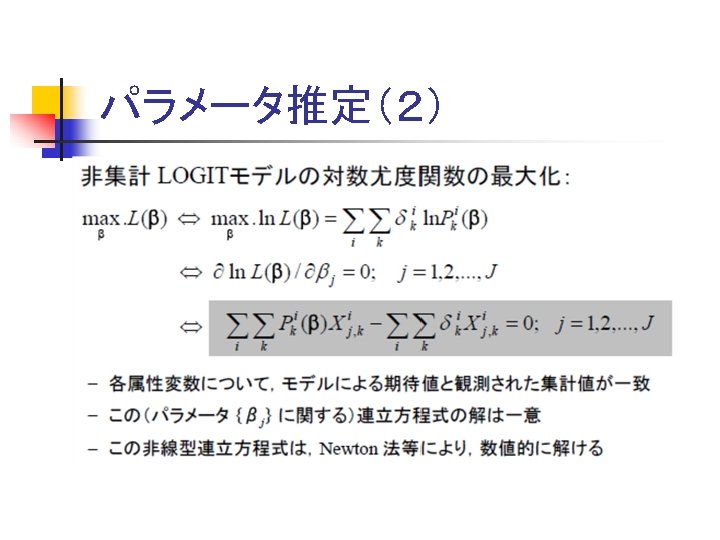
最尤法によるロジットモデルの推定 Maximum Likelihood Estimation 表 3. 15 バスの所要時間 表 3. 17 バスの所要費用 tBij c. Bij 1 2 3 1 5 11 130 140 180 2 10 12 12 2 140 130 220 3 14 16 7 3 180 220 130 単位:分 単位:円 表 3. 16 自動車の所要時 間 表 3. 18 自動車の所要費用 t. Cij c. Cij 1 2 3 1 21 45 58 1 3 8 10 2 45 42 60 2 8 7 11 3 58 60 19 3 10 11 3 単位:分 単位:円
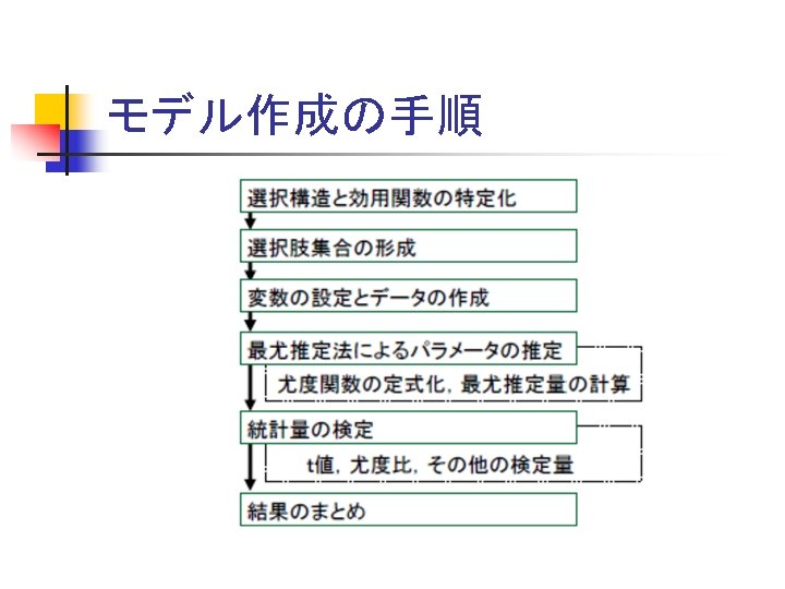
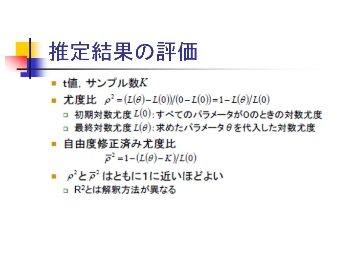
作成されたロジットモデル Estimated Logit model
Rにおける 尤度関数の定義と最大化 #対数尤度関数の定義 係数ベクトルxの関数と見なす. LL <- function (x){ vbus <- x[1] * tb + x[2] * cb vcar <- x[1] * tc + x[2] * cc + x[3] ppb <- 1/(1+exp(vcar - vbus)) ppc <- 1 - ppb return(sum(pb*log(ppb)+pc*log(ppc))) } #Optim関数で最大化を行い,結果をresに代入する.初期値は(0, 0, 0) b 0=c(0, 0, 0) res<-optim(b 0, LL, method = "BFGS", hessian = TRUE, control=list(fnscale=-1))
Rによる推定結果の表示 > res $par [1] -0. 081037584 -0. 004007811 0. 369193890 $value [1] -5. 047779 $counts function gradient 62 18 $convergence [1] 0 $message NULL $hessian [, 1] [, 2] [, 3] [1, ] -19. 628306 -613. 3939 5. 313007 [2, ] -613. 393875 -23980. 3173 196. 530577 [3, ] 5. 313007 196. 5306 -1. 681972
Rによる非集計最尤法の推定 Maximum Likelihood by R n 完全非集計データ(1サンプル 1行)の時 Pure disaggregate data (one line for one sample) n n glm(従属変数~独立変数1+・・・+独立変 数n, family=binomial(link=“logit”)) 従属変数が比率の場合 Share data n glm(従属変数~独立変数1+・・・+独立変 数n, family=quasibinomial(link=“logit”))
Rによる最尤法での推定 比率を説明する場合(share data) ans 2 <- glm(pc ~ tsa+csa, family=quasibinomial(link="logit")) summary(ans 2) Call: glm(formula = pc ~ tsa + csa, family = quasibinomial(link = "logit")) Deviance Residuals: Min 1 Q Median 3 Q Max -0. 008856 -0. 007615 -0. 002659 0. 007188 0. 013667 Coefficients: Estimate Std. Error t value Pr(>|t|) (Intercept) 0. 3991916 0. 0446219 8. 946 0. 000109 *** tsa -0. 0787542 0. 0060030 -13. 119 1. 21 e-05 *** csa -0. 0038095 0. 0003174 -12. 001 2. 03 e-05 *** --Signif. codes: 0 ‘***’ 0. 001 ‘**’ 0. 01 ‘*’ 0. 05 ‘. ’ 0. 1 ‘ ’ 1 (Dispersion parameter for quasibinomial family taken to be 0. 0001007740)
各個人の選択を説明する場合 Rにより,個人ごとのデータを作成 nb <- c(39, 11, 16, 22, 31, 15, 21, 25, 50) nc <- c(104, 28, 51, 61, 94, 63, 62, 73, 155) nn <- nb + nc nnf <-numeric(length=10) for (i in 1: 9){ nnf[i+1]=nnf[i]+nn[i] } chc <- numeric(length=nnf[10]-1) tim <- numeric(length=nnf[10]-1) cst <- numeric(length=nnf[10]-1) for (i in 1: 9){ chc[nnf[i]: (nnf[i]+nn[i]-1)] <- c(rep(1, nb[i]), rep(0, nc[i])) tim[nnf[i]: (nnf[i]+nn[i]-1)] <- rep((tb[i]-tc[i]), nn[i]) cst[nnf[i]: (nnf[i]+nn[i]-1)] <- rep((cb[i]-cc[i]), nn[i])
各個人の選択を説明する場合 pure disaggregate data ans 3 <- glm(chc ~ tim+cst, family=binomial(link="logit")) summary(ans 3) Call: glm(formula = chc ~ tim + cst, family = binomial(link = "logit")) Deviance Residuals: Min 1 Q Median 3 Q Max -0. 8215 -0. 7630 -0. 7470 -0. 1019 1. 8016 Coefficients: Estimate Std. Error z value Pr(>|z|) (Intercept) -0. 385889 0. 507795 -0. 760 0. 447 tim -0. 079514 0. 061803 -1. 287 0. 198 cst -0. 003873 0. 003465 -1. 118 0. 264 (Dispersion parameter for binomial family taken to be 1) Null deviance: 1034. 7 on 919 degrees of freedom Residual deviance: 1032. 4 on 917 degrees of freedom AIC: 1038. 4 Number of Fisher Scoring iterations: 4
ニュートン・ラプソン法 Newton Raphson Method
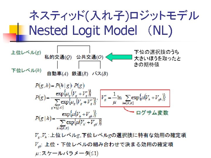
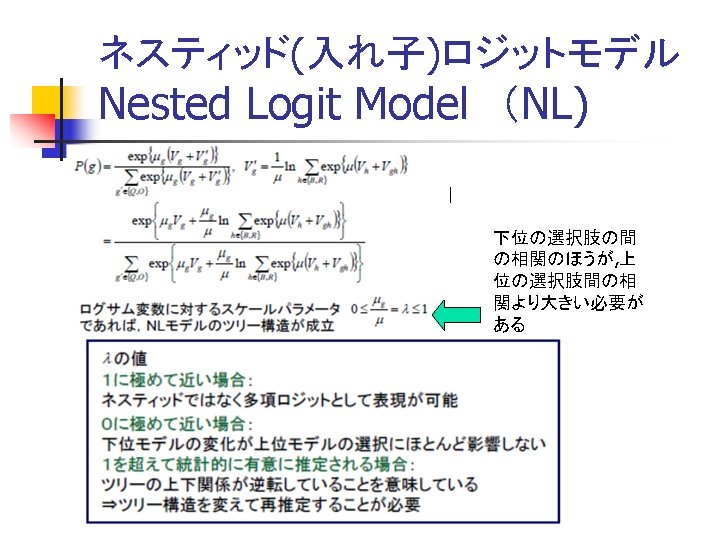
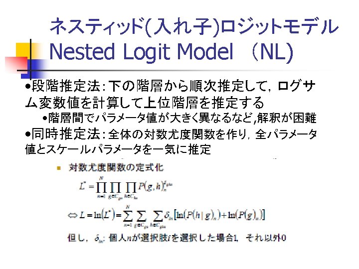
多項ロジットモデル Multinomial Logit Model
多項ロジットモデル用のデータ( 愛媛大学作成:)ehime. csv SEQ, 選択, 年齢, 保有台数, 鉄道可能性, 時間, 費用, バス可能性, 時間, 費用, 4輪可能性, 時間, 費用 3869, 1, 7, 5, 1, 37. 2 , 250, 1, 129. 0 , 850, 1, 25. 61, 120. 61 7447, 1, 7, 5, 1, 37. 2 , 250, 1, 121. 3 , 1174. 33, 1, 25. 61, 120. 61 7924, 1, 7, 5, 1, 42. 1 , 230, 1, 148. 3 , 960, 1, 29. 85, 142. 34 2460, 1, 5, 5, 1, 39. 0 , 230, 1, 106. 6 , 970, 1, 37. 06, 177. 84 3800, 1, 5, 5, 1, 39. 0 , 230, 1, 91. 3 , 850, 1, 37. 06, 177. 84 3347, 1, 3, 5, 1, 22. 0 , 140, 1, 77. 9 , 300, 1, 9. 41, 34. 04 4143, 1, 3, 5, 1, 22. 0 , 140, 1, 77. 9 , 300, 1, 9. 41, 34. 04 2529, 1, 1, 5, 1, 45. 0 , 320, 1, 94. 8 , 910, 1, 34. 42, 165. 4 4985, 1, 1, 5, 1, 45. 0 , 320, 1, 128. 5 , 1050, 1, 34. 42, 165. 39 6424, 1, 6, 4, 1, 83. 3 , 570, 1, 179. 8 , 1604. 61, 1, 62. 26, 511. 51 7791, 1, 6, 4, 1, 83. 3 , 570, 1, 172. 0 , 1720, 1, 62. 26, 511. 51 1498, 1, 5, 4, 1, 43. 6 , 650, 1, 169. 3 , 1932. 33, 1, 77. 59, 400. 49 1962, 1, 5, 4, 1, 54. 1 , 609, 1, 136. 0 , 1182. 28, 1, 61. 78, 313. 43 2367, 1, 5, 4, 1, 120. 3 , 1100, 1, 112. 2 , 1449. 06, 1, 60. 44, 306. 36 2369, 1, 5, 4, 1, 120. 3 , 1100, 1, 112. 2 , 1449. 06, 1, 60. 44, 306. 36 3985, 1, 5, 4, 1, 54. 1 , 609, 1, 134. 2 , 1182. 28, 1, 61. 78, 313. 43 4307, 1, 5, 4, 1, 43. 6 , 650, 1, 183. 8 , 2082. 33, 1, 77. 59, 400. 49 4931, 1, 5, 4, 1, 155. 0 , 1100, 1, 143. 1 , 1449. 06, 1, 60. 44, 306. 36 4932, 1, 5, 4, 1, 155. 0 , 1100, 1, 143. 1 , 1449. 06, 1, 60. 44, 306. 36 4701, 1, 1, 4, 1, 54. 7 , 320, 1, 105. 9 , 1020, 1, 31. 65, 160. 45 5774, 1, 1, 4, 1, 29. 7 , 180, 1, 67. 4 , 450, 1, 14. 63, 61. 37 6840, 1, 1, 4, 1, 29. 7 , 180, 1, 97. 8 , 450, 1, 14. 63, 61. 37 7242, 1, 1, 4, 1, 54. 7 , 320, 1, 98. 9 , 882. 17, 1, 31. 65, 160. 45 2368, 1, 7, 3, 1, 120. 3 , 1100, 1, 112. 2 , 1449. 06, 1, 60. 44, 306. 36 3309, 1, 7, 3, 1, 75. 7 , 570, 1, 167. 2 , 1460, 1, 58. 17, 497. 65 4662, 1, 7, 3, 1, 18. 0 , 140, 1, 70. 4 , 160, 1, 6. 81, 20. 01 4830, 1, 7, 3, 1, 35. 3 , 296, 1, 95. 3 , 440, 1, 20. 37, 92. 23 4933, 1, 7, 3, 1, 155. 0 , 1100, 1, 143. 1 , 1449. 06, 1, 60. 44, 306. 36 4980, 1, 7, 3, 1, 33. 7 , 190, 1, 125. 1 , 800, 1, 22. 24, 102. 38
多項ロジットモデルの最尤法プ ログラム(愛媛大学作成:) ### Multi Nomial Logit (MNL) estimation program (Original code by EHIME University) ###データファイルの読み込み Data<-read. csv("ehime. csv", header=T) hh<-nrow(Data) ##データ数: Data の行数を数える print(hh) ch<- 3 ##今回用いる選択肢の数 b 0<-c(0, 0, 0, 0) Srail <- sum(Data[, 14]== 1); Sbus <- sum(Data[, 14]== 2); Scar <- sum(Data[, 14]== 3) cat("rail: ", Srail, " bus: ", Sbus, " car: ", Scar, "n") ## Logit model の対数尤度関数の定義 fr <- function(x) { LL=0 ##効用の計算 rail <- x[1]*Data[, 6]/100 + x[2]*Data[, 7]/100 + x[5]*matrix(1, nrow =hh, ncol=1) bus <- x[1]*Data[, 9]/100 + x[2]*Data[, 10]/100 + x[3]*(Data[, 3]>=6) + x[6]*matrix(1, nrow=hh, ncol=1) car <- x[1]*Data[, 12]/100 + x[2]*Data[, 13]/100 + x[4]*(Data[, 4]>=2) ##効用の指数化 Erail <- exp(rail)*Data[, 5] Ebus <- exp(bus )*Data[, 8] Ecar <- exp(car )*Data[, 11] PPrail <- Erail/(Erail+Ebus+Ecar) PPbus <- Ebus /(Erail+Ebus+Ecar) PPcar <- Ecar /(Erail+Ebus+Ecar) ##選択結果の確率のみを有効化 Prail <- (PPrail!=0)*PPrail + (PPrail==0) Pbus <- (PPbus !=0)*PPbus + (PPbus ==0) Pcar <- (PPcar !=0)*PPcar + (PPcar ==0) ##選択結果 Crail <- Data[, 14]== 1
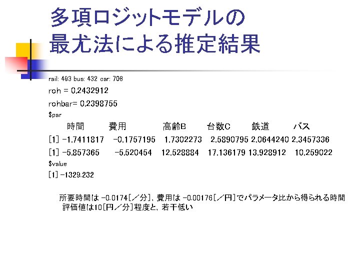
多項ロジットモデルの 最尤法による推定結果 rail: 493 bus: 432 car: 708 roh = 0. 2432912 rohbar= 0. 2398755 $par [1] -1. 7411817 -0. 1757195 1. 7302273 2. 5890795 2. 0644240 2. 3457336 $value [1] -1329. 232 $counts function gradient 38 14 $convergence [1] 0 $message NULL $hessian [, 1] [, 2] [, 3] [, 4] [, 5] [, 6] [1, ] -80. 15815 -538. 9584 -67. 42988 65. 52220 27. 40143 -114. 7780 [2, ] -538. 95843 -4708. 3230 -493. 74059 503. 37025 123. 55640 -800. 5406 [3, ] -67. 42988 -493. 7406 -127. 96682 31. 64655 79. 67259 -127. 9668 [4, ] 65. 52220 503. 3703 31. 64655 -214. 17601 136. 44173 77. 7343 [5, ] 27. 40143 123. 5564 79. 67259 136. 44173 -293. 24442 123. 6202 [6, ] -114. 77804 -800. 5406 -127. 96682 77. 73429 123. 62021 -224. 7471 [1] -5. 857365 -5. 520454 12. 528884 17. 136179 13. 928912 10. 259022
多項ロジットモデル (パッケージ) Multinomial Logit Model install. packages("mlogit") library("mlogit") Dehime<-read. csv("ehime. csv", header=T) Ehime <-mlogit. data(Dehime, varying=c(5: 13), shape="wide", choice="choice") #MNL without constant term summary(mlogit(choice~time+cost-1, data=Ehime)) #MNL with constant term summary(mlogit(choice~time+cost, data=Ehime))
多項ロジットモデル(定数項なし) Multinomial Logit Model Call: mlogit(formula = Choice ~ time + cost - 1, data = Ehime) Frequencies of alternatives: bus car rail 0. 26454 0. 43356 0. 30190 Newton-Raphson maximisation gradient close to zero. May be a solution 5 iterations, 0 h: 0 m: 0 s g'(-H)^-1 g = 7. 47 E-31 Coefficients : Estimate Std. Error t-value Pr(>|t|) time -0. 00329405 0. 00197725 -1. 6660 0. 0957185. cost -0. 00096882 0. 00025323 -3. 8259 0. 0001303 *** --Signif. codes: 0 ‘***’ 0. 001 ‘**’ 0. 01 ‘*’ 0. 05 ‘. ’ 0. 1 ‘ ’ 1 Log-Likelihood: -1715. 7
多項ロジットモデル(定数項あり) Multinomial Logit Model Call: mlogit(formula = Choice ~ time + cost, data = Ehime) Frequencies of alternatives: bus car rail 0. 26454 0. 43356 0. 30190 Newton-Raphson maximisation gradient close to zero. May be a solution 5 iterations, 0 h: 0 m: 0 s g'(-H)^-1 g = 9. 17 E-26 Coefficients : Estimate Std. Error t-value Pr(>|t|) altcar -1. 07985435 0. 14856671 -7. 2685 3. 635 e-13 altrail -0. 95903599 0. 11625041 -8. 2497 2. 220 e-16 time -0. 01607098 0. 00261456 -6. 1467 7. 910 e-10 cost -0. 00119568 0. 00027125 -4. 4081 1. 043 e-05 Log-Likelihood: -1680. 5 Mc. Fadden R^2: 0. 68776 Likelihood ratio test : chisq = 152. 13 (p. value=< 2. 22 e-16 *** ***
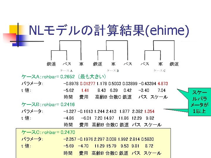
ネスティッドロジットモデルの最尤 法プログラム(愛媛大学作成:) ### Nested Logit estimation program (Original code by EHIME University) ###データファイルの読み込み Data<-read. csv(“ehime. csv", header=T) hh<-nrow(Data) ##データ数: Data の行数を数える print(hh) ch<- 3 ##今回用いる選択肢の数 b 0<-c(0, 0, 0, 1) ##初期パラメータ値(全て 0) ## サンプルにおける各選択肢のシェア Srail <- sum(Data[, 2]==“rail”); Sbus <- sum(Data[, 2]==“ bus”); Scar <- sum(Data[, 2]==“car”) cat("rail: ", Srail, " bus: ", Sbus, " car: ", Scar, "n") ## Logit model の対数尤度関数の定義 fr <- function(x) { LL=0 ##効用の計算 rail <- x[1]*Data[, 6]/100 + x[2]*Data[, 7]/100 + x[5]*matrix(1, nrow =hh, ncol=1) bus <- x[1]*Data[, 9]/100 + x[2]*Data[, 10]/100 + x[3]*(Data[, 3]>=6) + x[6]*matrix(1, nrow =hh, ncol=1) car <- x[1]*Data[, 12]/100 + x[2]*Data[, 13]/100 + x[4]*(Data[, 4]>=2) ##効用の指数化 Erail <- exp(rail)*Data[, 5] Ebus <- exp(bus )*Data[, 8] Ecar <- exp(car )*Data[, 11]