MATH 1046 Elementary row operations and row echelon

MATH 1046 Elementary row operations and row echelon form (Sections 2. 2 – Direct methods of solving linear systems) Alex Karassev

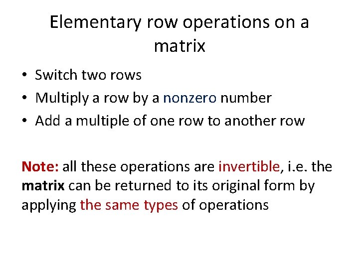
Elementary row operations on a matrix • Switch two rows • Multiply a row by a nonzero number • Add a multiple of one row to another row Note: all these operations are invertible, i. e. the matrix can be returned to its original form by applying the same types of operations

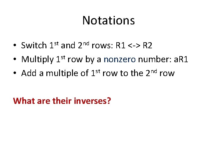
Notations • Switch 1 st and 2 nd rows: R 1 <-> R 2 • Multiply 1 st row by a nonzero number: a. R 1 • Add a multiple of 1 st row to the 2 nd row What are their inverses?

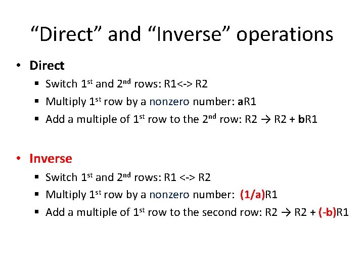
“Direct” and “Inverse” operations • Direct § Switch 1 st and 2 nd rows: R 1<-> R 2 § Multiply 1 st row by a nonzero number: a. R 1 § Add a multiple of 1 st row to the 2 nd row: R 2 → R 2 + b. R 1 • Inverse § Switch 1 st and 2 nd rows: R 1 <-> R 2 § Multiply 1 st row by a nonzero number: (1/a)R 1 § Add a multiple of 1 st row to the second row: R 2 → R 2 + (-b)R 1

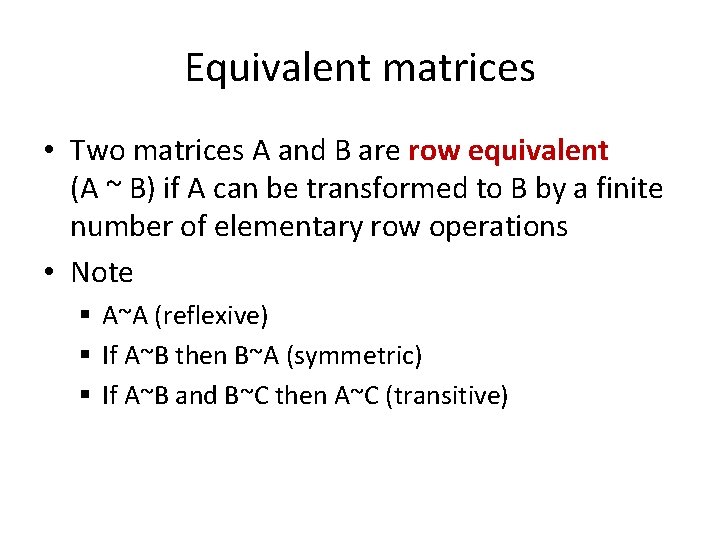
Equivalent matrices • Two matrices A and B are row equivalent (A ~ B) if A can be transformed to B by a finite number of elementary row operations • Note § A~A (reflexive) § If A~B then B~A (symmetric) § If A~B and B~C then A~C (transitive)

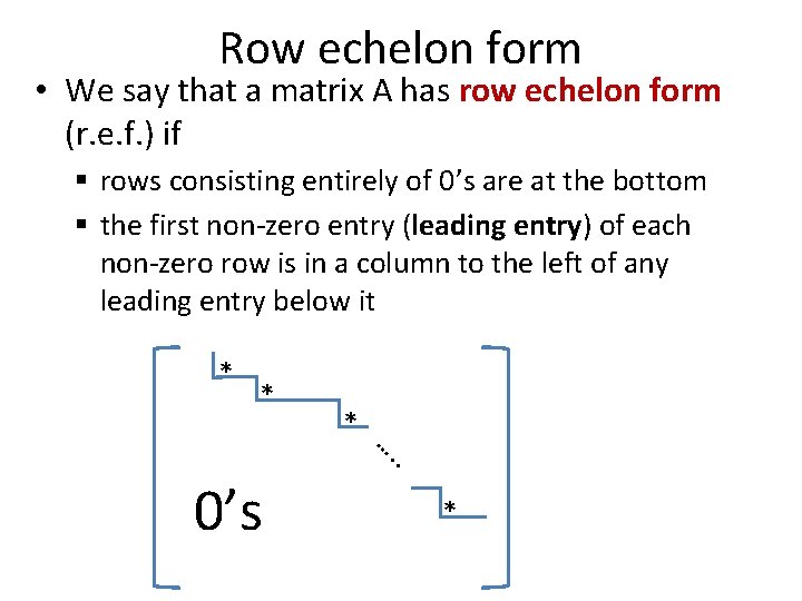
Row echelon form • We say that a matrix A has row echelon form (r. e. f. ) if § rows consisting entirely of 0’s are at the bottom § the first non-zero entry (leading entry) of each non-zero row is in a column to the left of any leading entry below it * * 0’s * …. . *

Theorem. Any matrix is equivalent to a matrix in a r. e. f.

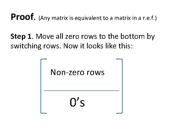
Proof. (Any matrix is equivalent to a matrix in a r. e. f. ) Step 1. Move all zero rows to the bottom by switching rows. Now it looks like this: Non-zero rows 0’s

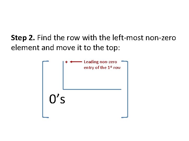
Step 2. Find the row with the left-most non-zero element and move it to the top: * 0’s Leading non-zero entry of the 1 st row

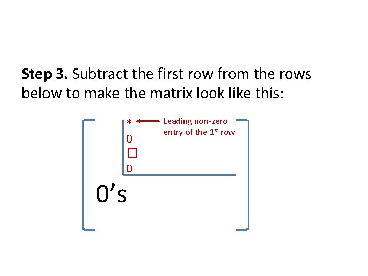
Step 3. Subtract the first row from the rows below to make the matrix look like this: * 0 � 0 0’s Leading non-zero entry of the 1 st row

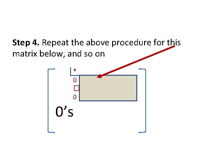
Step 4. Repeat the above procedure for this matrix below, and so on * 0 � 0 0’s

Theorem. Two matrices are row equivalent if and only if they can be transformed to the same row echelon form Proof. • Suppose first that A~B. Let C be the row echelon form of B, i. e. C is in r. e. f. and B~C. Then A~C, as required. • Conversely, suppose there exists C (in r. e. f. ) such that A~C and B~C. Then C~B and therefore A~B

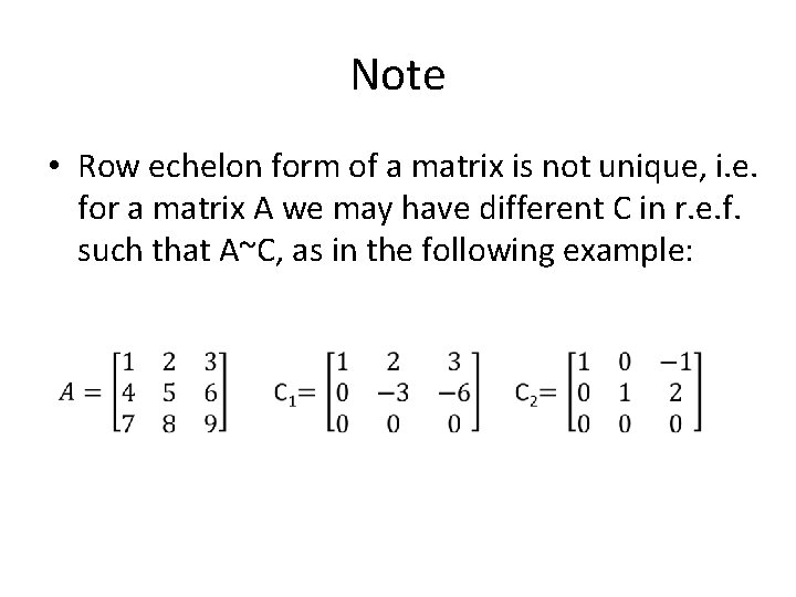
Note • Row echelon form of a matrix is not unique, i. e. for a matrix A we may have different C in r. e. f. such that A~C, as in the following example:

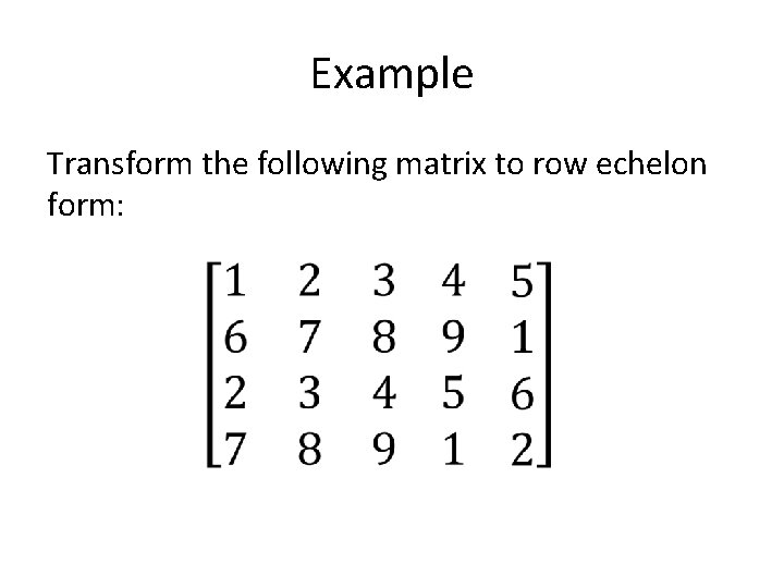
Example Transform the following matrix to row echelon form:

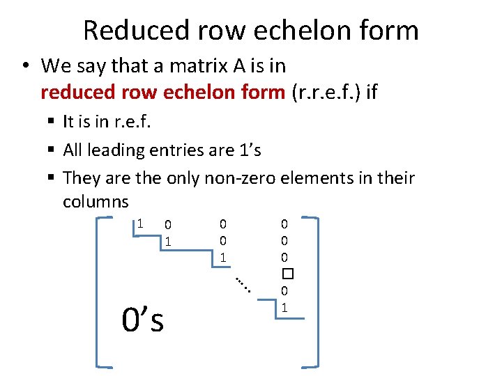
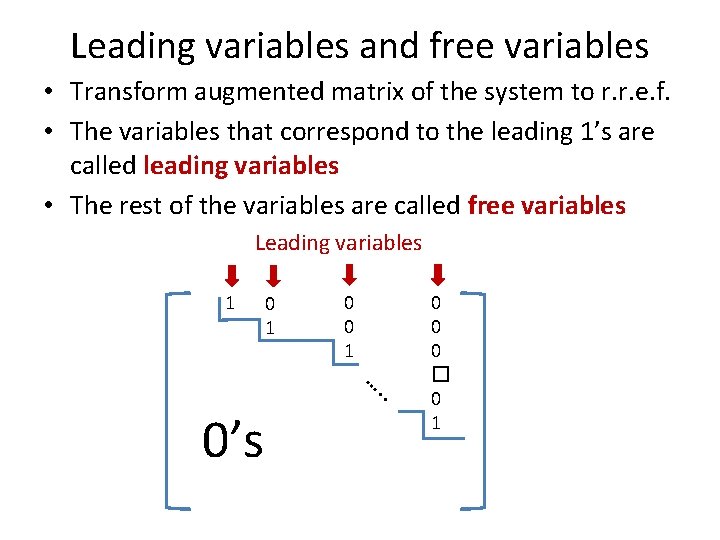
Reduced row echelon form • We say that a matrix A is in reduced row echelon form (r. r. e. f. ) if § It is in r. e. f. § All leading entries are 1’s § They are the only non-zero elements in their columns 1 0 0 1 …. . 0’s 0 0 0 � 0 1

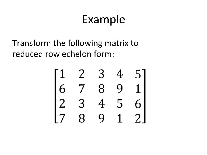
Example Transform the following matrix to reduced row echelon form:

Rank • Definition. The rank of a matrix A is the number of leading entries in (any of) its r. e. f. • Notation: rank(A)

Rank • Definition. The rank of a matrix A is the number of leading entries in (any of) its r. e. f. • Notation: rank(A) • Problem: why is rank(A) well-defined? i. e. can it happen that A~B and A~C, such that B and C are in r. e. f. but have different number of leading 1 s?

Rank • Definition. The rank of a matrix A is the number of leading entries in (any of) its r. e. f. • Notation: rank(A) • Problem: why is rank(A) well-defined? i. e. can it happen that A~B and A~C, such that B and C are in r. e. f. but have different number of leading zeroes? • We will show later that such thing cannot happen, and thus rank(A) is well-defined

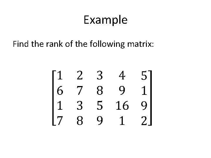
Example Find the rank of the following matrix:

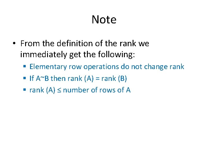
Note • From the definition of the rank we immediately get the following: § Elementary row operations do not change rank § If A~B then rank (A) = rank (B) § rank (A) ≤ number of rows of A

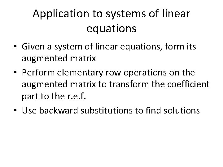
Application to systems of linear equations • Given a system of linear equations, form its augmented matrix • Perform elementary row operations on the augmented matrix to transform the coefficient part to the r. e. f. • Use backward substitutions to find solutions

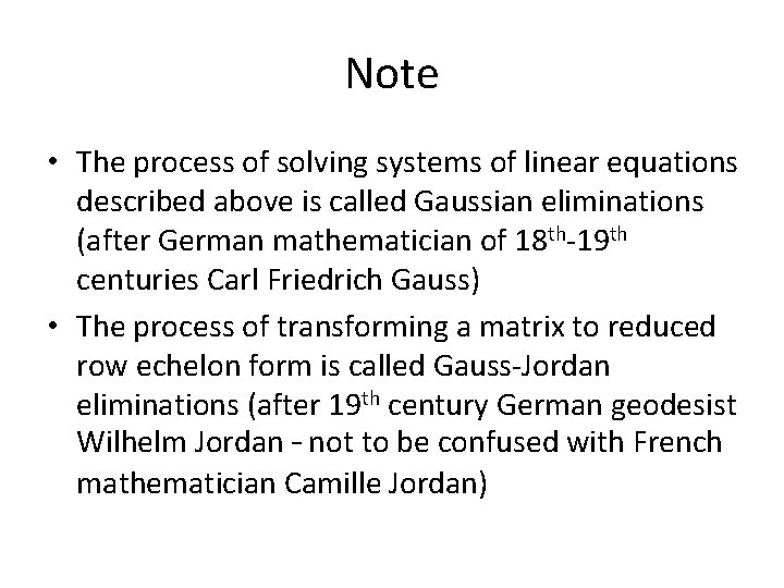
Note • The process of solving systems of linear equations described above is called Gaussian eliminations (after German mathematician of 18 th-19 th centuries Carl Friedrich Gauss) • The process of transforming a matrix to reduced row echelon form is called Gauss-Jordan eliminations (after 19 th century German geodesist Wilhelm Jordan – not to be confused with French mathematician Camille Jordan)

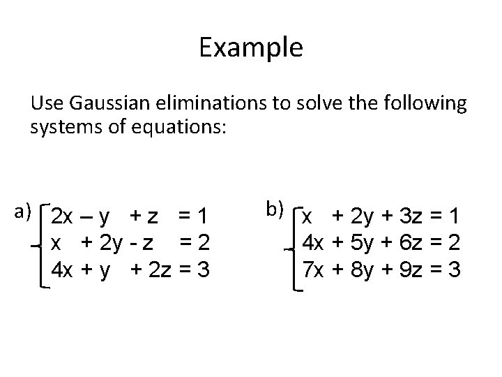
Example Use Gaussian eliminations to solve the following systems of equations: a) 2 x – y + z = 1 x + 2 y - z = 2 4 x + y + 2 z = 3 b) x + 2 y + 3 z = 1 4 x + 5 y + 6 z = 2 7 x + 8 y + 9 z = 3

We see that a linear system can have • No solutions • Exactly one solution • Infinitely many solutions

We see that a linear system can have • No solutions • Exactly one solution • Infinitely may solutions Definition. If a linear system has at least one solution it is called consistent. Otherwise (i. e. if it has no solutions) it is called inconsistent

Question • Can a consistent system have finitely many (but more than one) solutions?

Question • Can a consistent system have finitely many (but more than one) solutions? • We will show that the answer is no, i. e. we can have only three possibilities: § no solutions § exactly one solution § infinitely many solutions

Leading variables and free variables • Transform augmented matrix of the system to r. r. e. f. • The variables that correspond to the leading 1’s are called leading variables • The rest of the variables are called free variables Leading variables 1 0 0 1 …. . 0’s 0 0 0 � 0 1

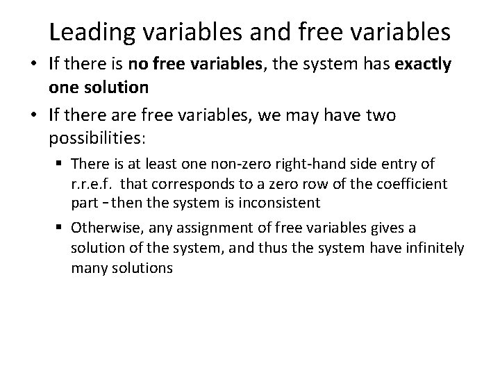
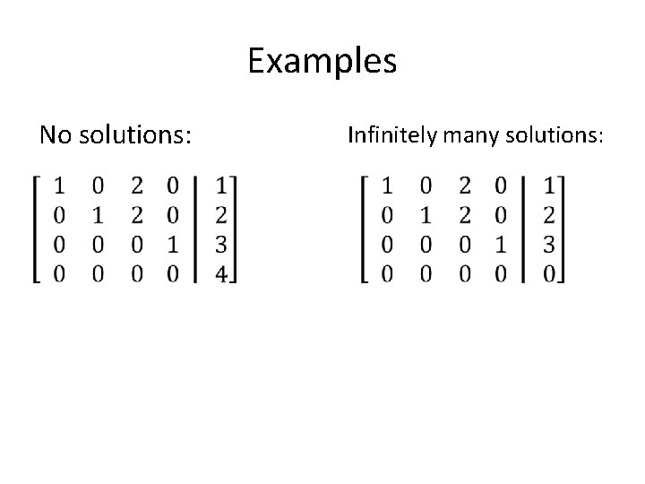
Leading variables and free variables • If there is no free variables, the system has exactly one solution • If there are free variables, we may have two possibilities: § There is at least one non-zero right-hand side entry of r. r. e. f. that corresponds to a zero row of the coefficient part – then the system is inconsistent § Otherwise, any assignment of free variables gives a solution of the system, and thus the system have infinitely many solutions

Examples No solutions: Infinitely many solutions:

Connection with rank • The number of the leading variables equals to the rank of A (the coefficient matrix) • Therefore, we get the Rank theorem rank (A) + (number of free variables) = n where n is the total number of variables, or equivalently the number of columns of A

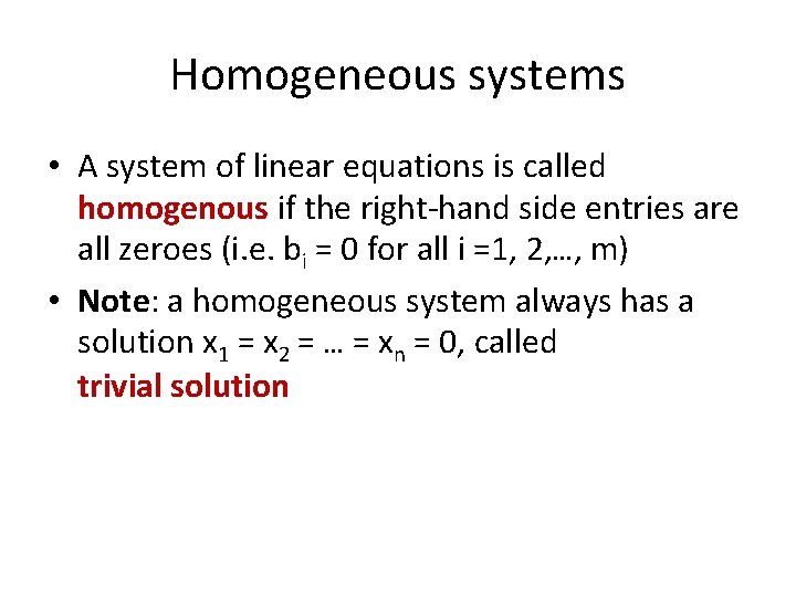
Homogeneous systems • A system of linear equations is called homogenous if the right-hand side entries are all zeroes (i. e. bi = 0 for all i =1, 2, …, m) • Note: a homogeneous system always has a solution x 1 = x 2 = … = xn = 0, called trivial solution

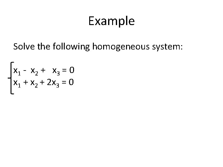
Example Solve the following homogeneous system: x 1 - x 2 + x 3 = 0 x 1 + x 2 + 2 x 3 = 0

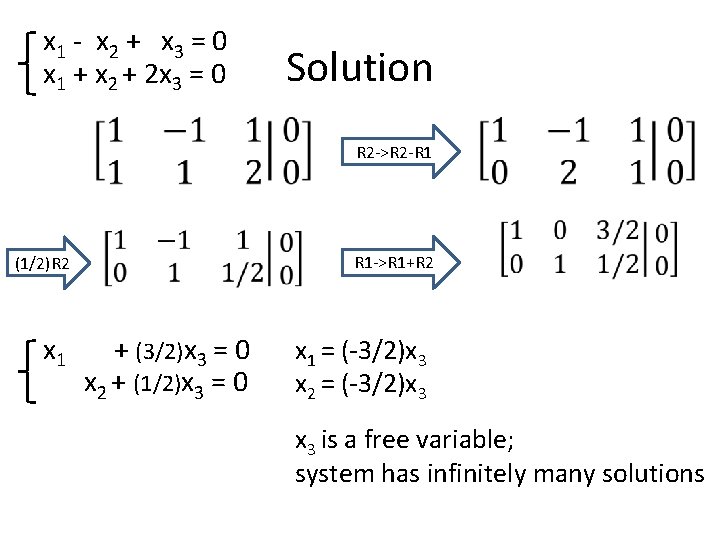
x 1 - x 2 + x 3 = 0 x 1 + x 2 + 2 x 3 = 0 Solution R 2 ->R 2 -R 1 R 1 ->R 1+R 2 (1/2)R 2 x 1 + (3/2)x 3 = 0 x 2 + (1/2)x 3 = 0 x 1 = (-3/2)x 3 x 2 = (-3/2)x 3 is a free variable; system has infinitely many solutions

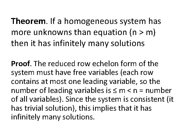
Theorem. If a homogeneous system has more unknowns than equation (n > m) then it has infinitely many solutions Proof. The reduced row echelon form of the system must have free variables (each row contains at most one leading variable, so the number of leading variables is ≤ m < n = number of all variables). Since the system is consistent (it has trivial solution), this implies that it has infinitely many solutions.