Magnetic Resonance Imaging Physical Principles Richard Watts D

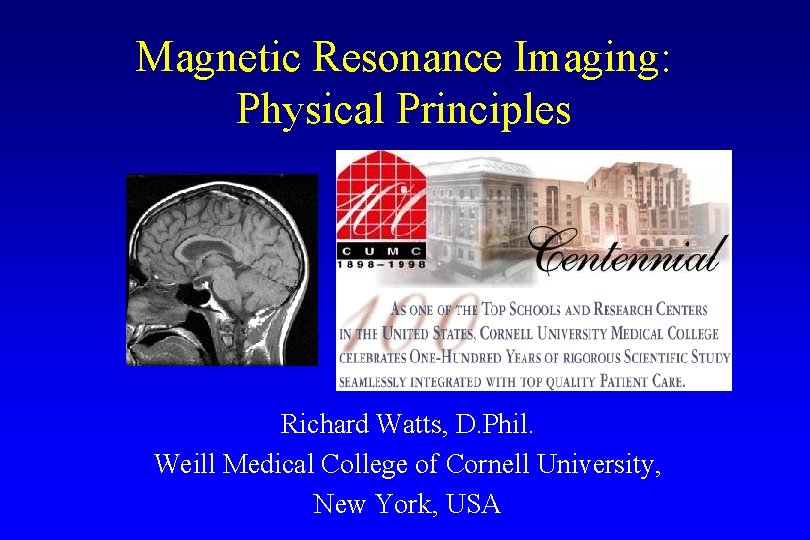
Magnetic Resonance Imaging: Physical Principles Richard Watts, D. Phil. Weill Medical College of Cornell University, New York, USA

Physics of MRI, Lecture 1 • Nuclear Magnetic Resonance – Nuclear spins – Spin precession and the Larmor equation – Static B 0 – RF excitation – RF detection • Fourier Transforms – Continuous Fourier Transform – Discrete Fourier Transform – Fourier properties – k-space representation in MRI • Spatial Encoding – Slice selective excitation – Frequency encoding – Phase encoding – Image reconstruction 10/24/2021 2

Bibliography • Magnetic Resonance Imaging – Physical Principles and Sequence Design. Haacke, Brown, Thompson, Venkatesan. Wiley 1999. • The Fourier Transform and It’s Applications. Bracewell. Mc. Graw-Hill 2000. • Medical books – simple, but little mathematical depth • Physics books – more depth, but more complicated • Web: http: //mri. med. cornell. edu/links. html 10/24/2021 3

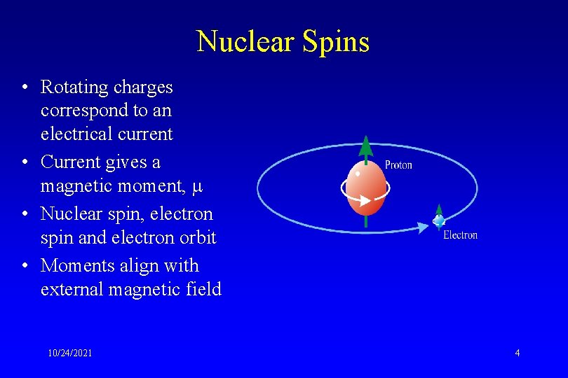
Nuclear Spins • Rotating charges correspond to an electrical current • Current gives a magnetic moment, • Nuclear spin, electron spin and electron orbit • Moments align with external magnetic field 10/24/2021 4

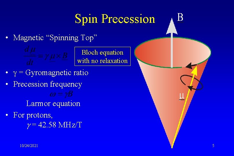
Spin Precession • Magnetic “Spinning Top” Bloch equation with no relaxation • = Gyromagnetic ratio • Precession frequency Larmor equation • For protons, = 42. 58 MHz/T 10/24/2021 5

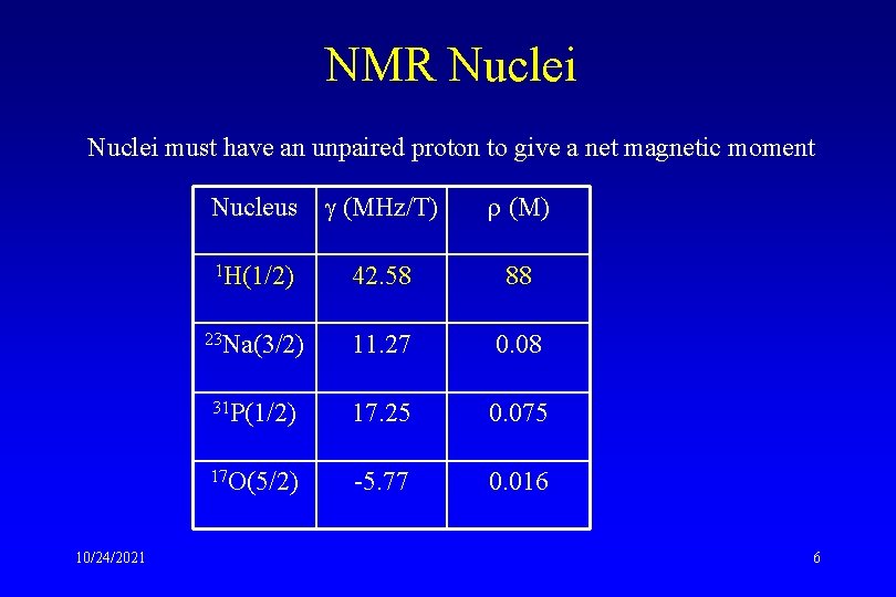
NMR Nuclei must have an unpaired proton to give a net magnetic moment 10/24/2021 Nucleus (MHz/T) (M) 1 H(1/2) 42. 58 88 23 Na(3/2) 11. 27 0. 08 31 P(1/2) 17. 25 0. 075 17 O(5/2) -5. 77 0. 016 6

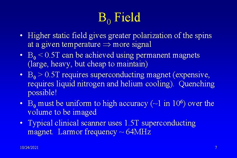
B 0 Field • Higher static field gives greater polarization of the spins at a given temperature more signal • B 0 < 0. 5 T can be achieved using permanent magnets (large, heavy, but cheap to maintain) • B 0 > 0. 5 T requires superconducting magnet (expensive, requires liquid nitrogen and helium cooling). Quenching possible! • B 0 must be uniform to high accuracy (~1 in 106) over the volume to be imaged • Typical clinical scanner uses 1. 5 T superconducting magnet. Larmor frequency ~ 64 MHz 10/24/2021 7

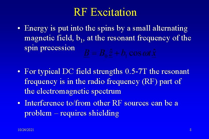
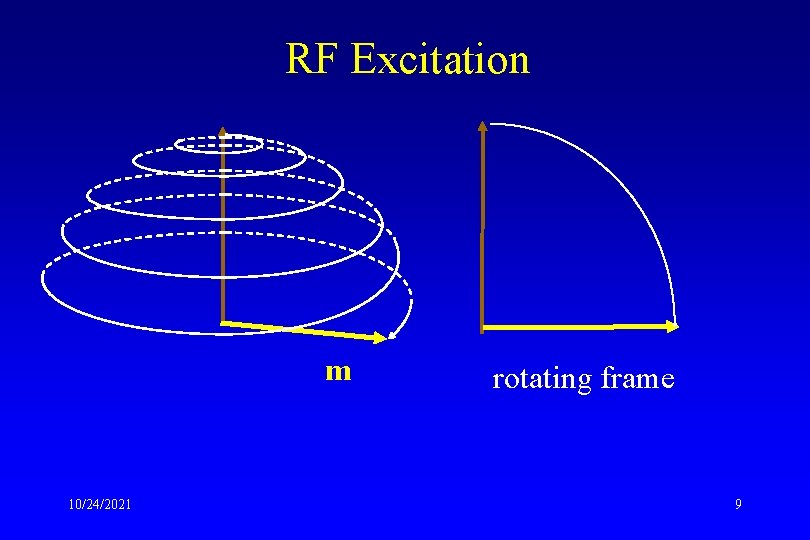
RF Excitation • Energy is put into the spins by a small alternating magnetic field, b 1, at the resonant frequency of the spin precession • For typical DC field strengths 0. 5 -7 T the resonant frequency is in the radio frequency (RF) part of the electromagnetic spectrum • Interference to/from other RF sources can be a problem – requires shielding 10/24/2021 8

RF Excitation m 10/24/2021 rotating frame 9

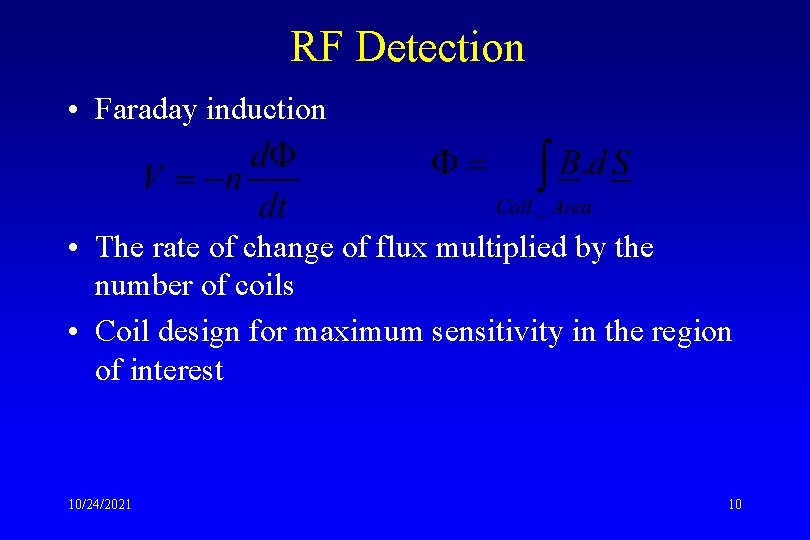
RF Detection • Faraday induction • The rate of change of flux multiplied by the number of coils • Coil design for maximum sensitivity in the region of interest 10/24/2021 10

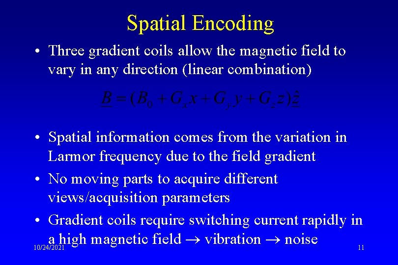
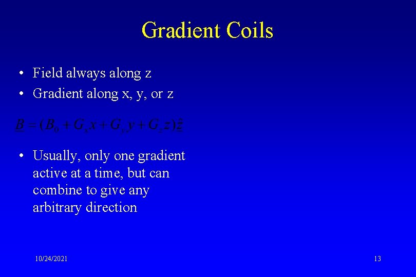
Spatial Encoding • Three gradient coils allow the magnetic field to vary in any direction (linear combination) • Spatial information comes from the variation in Larmor frequency due to the field gradient • No moving parts to acquire different views/acquisition parameters • Gradient coils require switching current rapidly in a high magnetic field vibration noise 10/24/2021 11

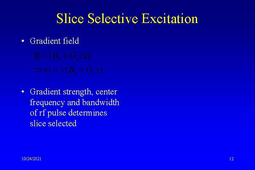
Slice Selective Excitation • Gradient field • Gradient strength, center frequency and bandwidth of rf pulse determines slice selected 10/24/2021 12

Gradient Coils • Field always along z • Gradient along x, y, or z • Usually, only one gradient active at a time, but can combine to give any arbitrary direction 10/24/2021 13

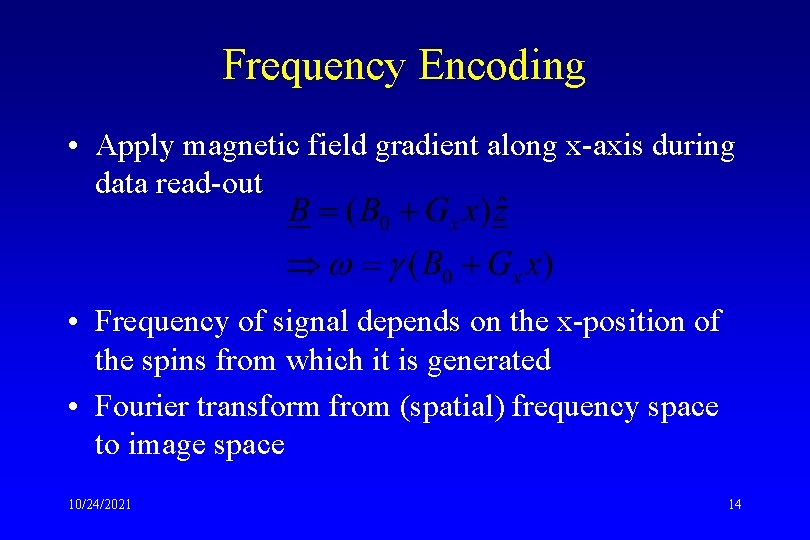
Frequency Encoding • Apply magnetic field gradient along x-axis during data read-out • Frequency of signal depends on the x-position of the spins from which it is generated • Fourier transform from (spatial) frequency space to image space 10/24/2021 14

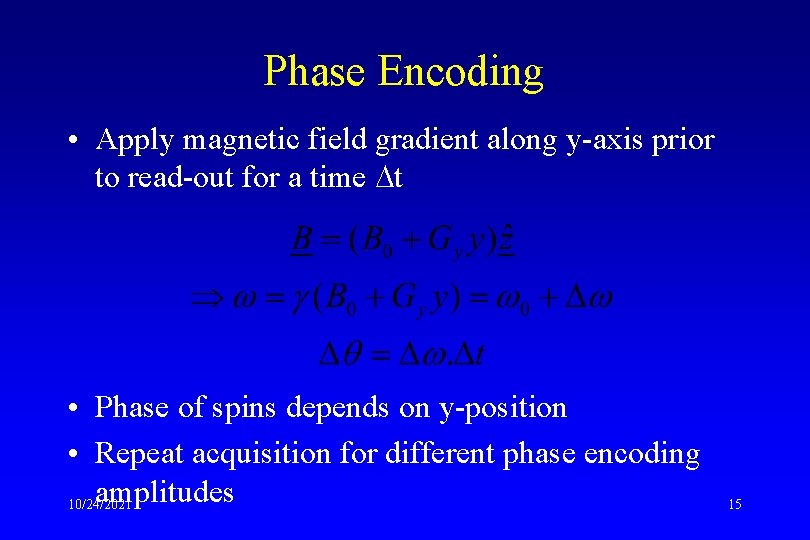
Phase Encoding • Apply magnetic field gradient along y-axis prior to read-out for a time t • Phase of spins depends on y-position • Repeat acquisition for different phase encoding amplitudes 10/24/2021 15

Image Reconstruction • Spins from all positions (voxels) contribute signals to each measurement (sample) • The frequency and phase of the signal from each voxel is determined by its spatial position • How do we form an image? Fourier Transforms! 10/24/2021 16

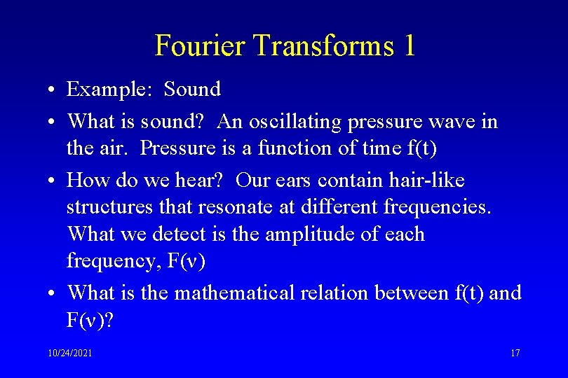
Fourier Transforms 1 • Example: Sound • What is sound? An oscillating pressure wave in the air. Pressure is a function of time f(t) • How do we hear? Our ears contain hair-like structures that resonate at different frequencies. What we detect is the amplitude of each frequency, F(ν) • What is the mathematical relation between f(t) and F(ν)? 10/24/2021 17

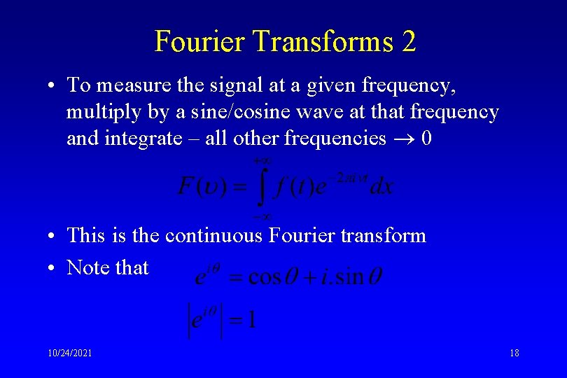
Fourier Transforms 2 • To measure the signal at a given frequency, multiply by a sine/cosine wave at that frequency and integrate – all other frequencies 0 • This is the continuous Fourier transform • Note that 10/24/2021 18

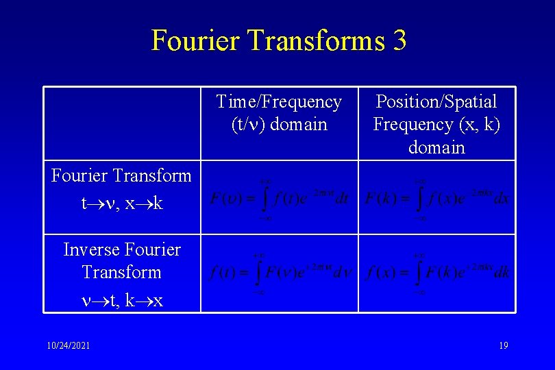
Fourier Transforms 3 Time/Frequency (t/ ) domain Position/Spatial Frequency (x, k) domain Fourier Transform t , x k Inverse Fourier Transform t, k x 10/24/2021 19

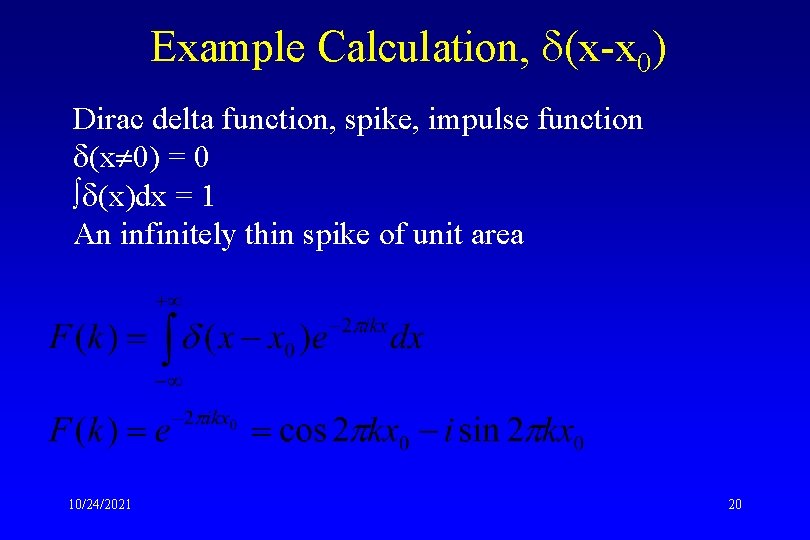
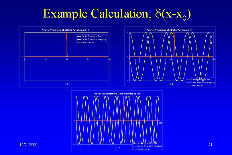
Example Calculation, (x-x 0) Dirac delta function, spike, impulse function (x 0) = 0 ò (x)dx = 1 An infinitely thin spike of unit area 10/24/2021 20

Example Calculation, (x-x 0) 10/24/2021 21

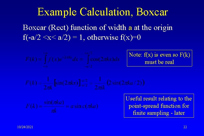
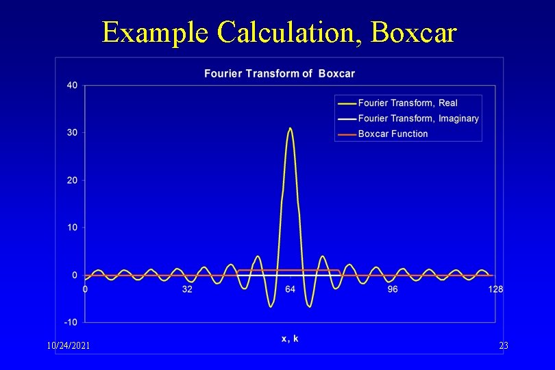
Example Calculation, Boxcar (Rect) function of width a at the origin f(-a/2 <x< a/2) = 1, otherwise f(x)=0 Note: f(x) is even so F(k) must be real Useful result relating to the point-spread function for finite sampling - later 10/24/2021 22

Example Calculation, Boxcar 10/24/2021 23

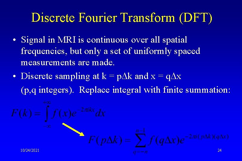
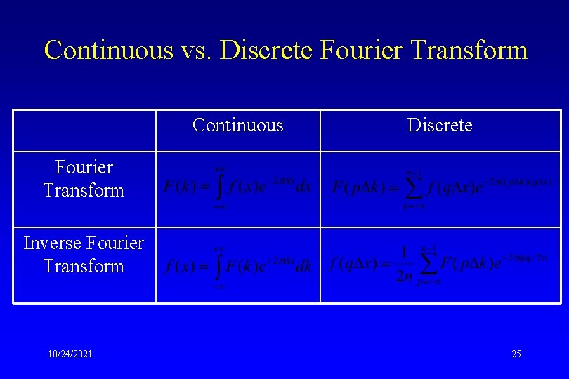
Discrete Fourier Transform (DFT) • Signal in MRI is continuous over all spatial frequencies, but only a set of uniformly spaced measurements are made. • Discrete sampling at k = p k and x = q x (p, q integers). Replace integral with finite summation: 10/24/2021 24

Continuous vs. Discrete Fourier Transform Continuous Discrete Fourier Transform Inverse Fourier Transform 10/24/2021 25

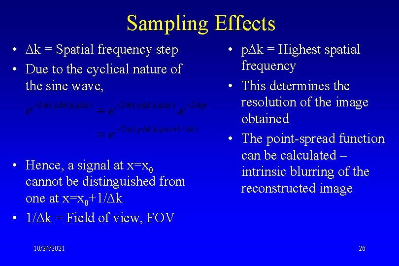
Sampling Effects • k = Spatial frequency step • Due to the cyclical nature of the sine wave, • Hence, a signal at x=x 0 cannot be distinguished from one at x=x 0+1/ k • 1/ k = Field of view, FOV 10/24/2021 • p k = Highest spatial frequency • This determines the resolution of the image obtained • The point-spread function can be calculated – intrinsic blurring of the reconstructed image 26

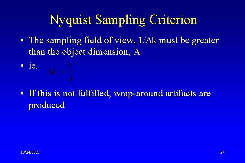
Nyquist Sampling Criterion • The sampling field of view, 1/ k must be greater than the object dimension, A • ie. • If this is not fulfilled, wrap-around artifacts are produced 10/24/2021 27

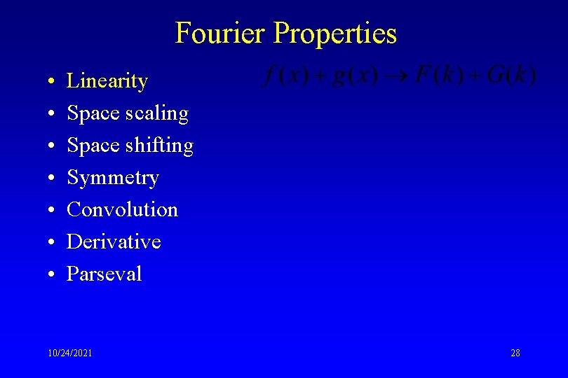
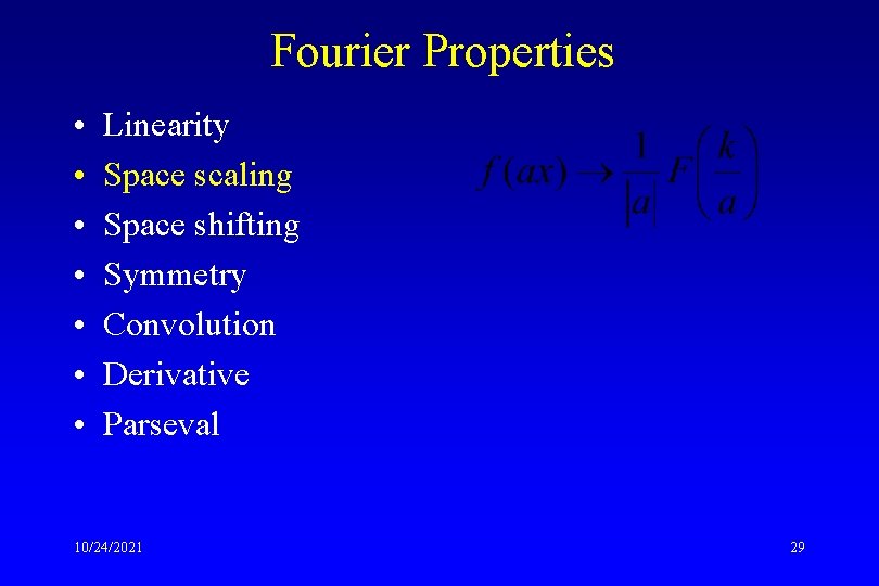
Fourier Properties • • Linearity Space scaling Space shifting Symmetry Convolution Derivative Parseval 10/24/2021 28

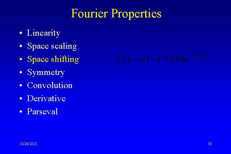
Fourier Properties • • Linearity Space scaling Space shifting Symmetry Convolution Derivative Parseval 10/24/2021 29

Fourier Properties • • Linearity Space scaling Space shifting Symmetry Convolution Derivative Parseval 10/24/2021 30

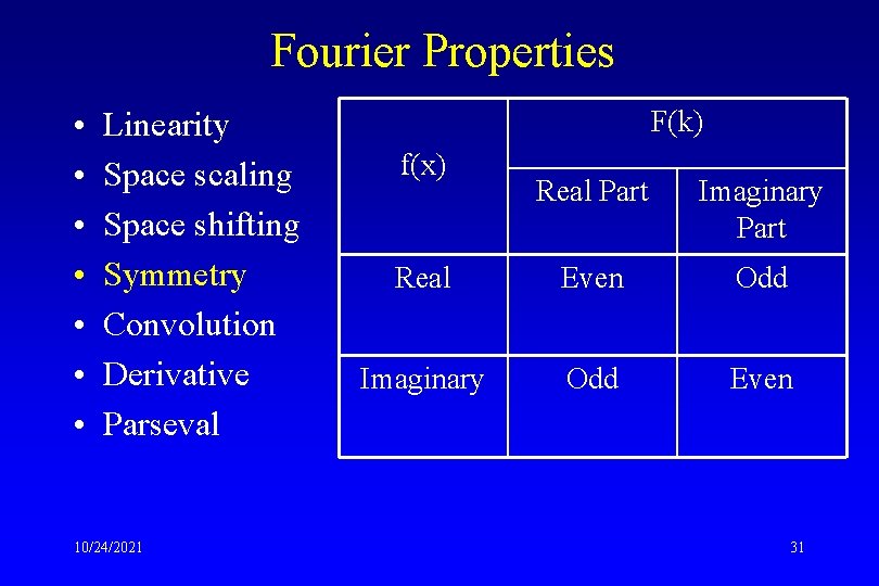
Fourier Properties • • Linearity Space scaling Space shifting Symmetry Convolution Derivative Parseval 10/24/2021 F(k) f(x) Real Part Imaginary Part Real Even Odd Imaginary Odd Even 31

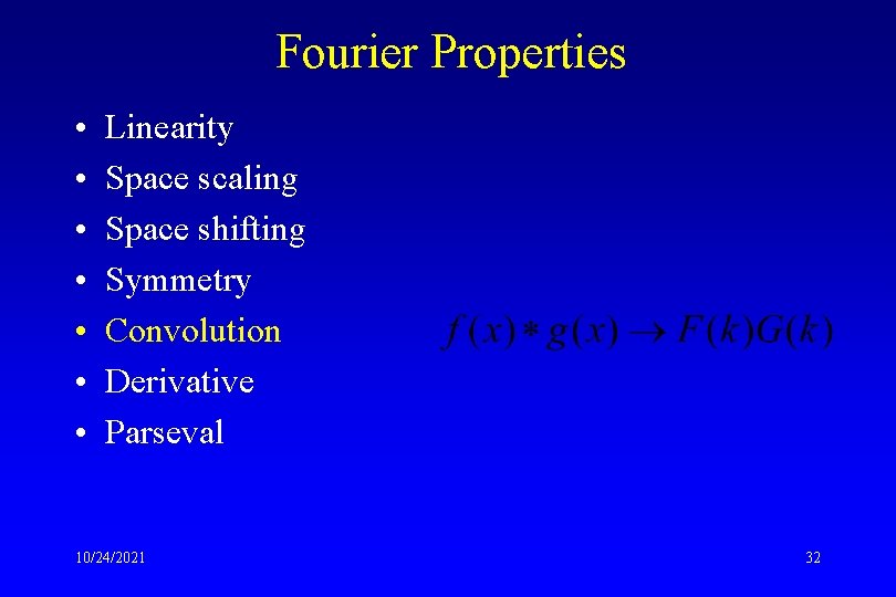
Fourier Properties • • Linearity Space scaling Space shifting Symmetry Convolution Derivative Parseval 10/24/2021 32

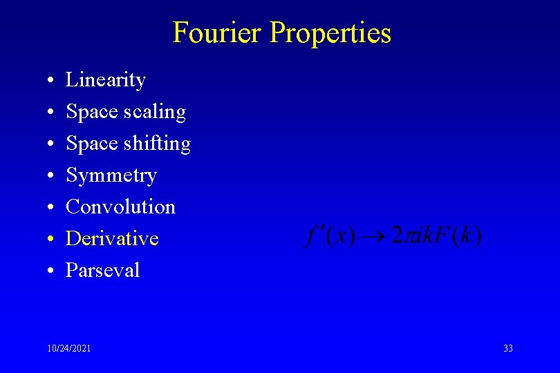
Fourier Properties • • Linearity Space scaling Space shifting Symmetry Convolution Derivative Parseval 10/24/2021 33

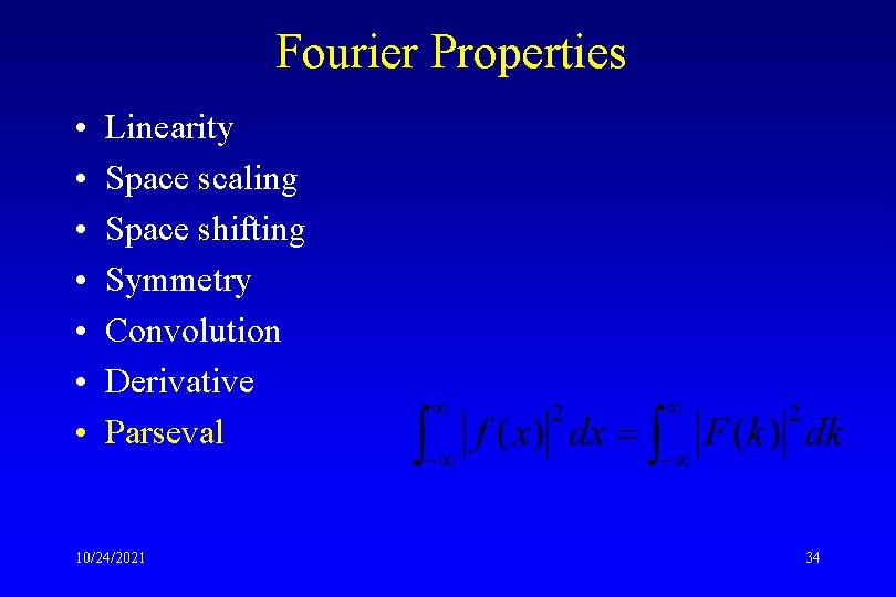
Fourier Properties • • Linearity Space scaling Space shifting Symmetry Convolution Derivative Parseval 10/24/2021 34

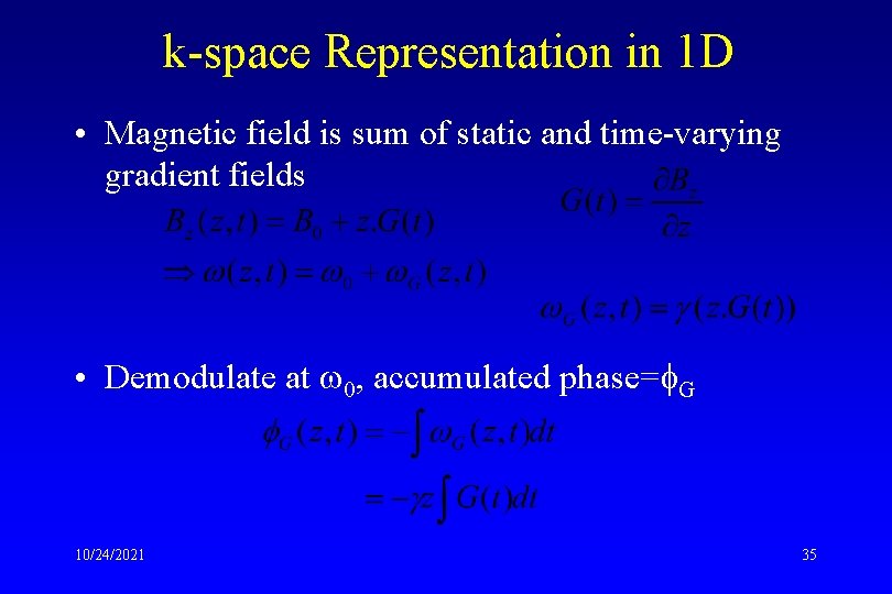
k-space Representation in 1 D • Magnetic field is sum of static and time-varying gradient fields • Demodulate at 0, accumulated phase= G 10/24/2021 35

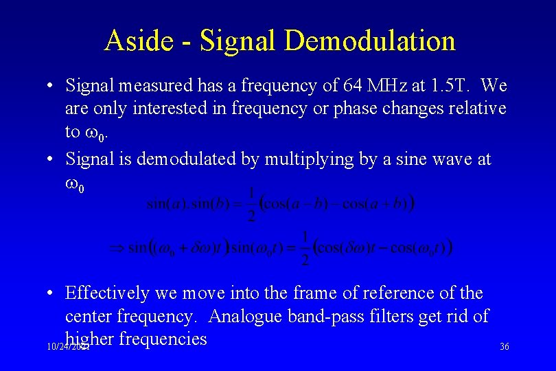
Aside - Signal Demodulation • Signal measured has a frequency of 64 MHz at 1. 5 T. We are only interested in frequency or phase changes relative to 0. • Signal is demodulated by multiplying by a sine wave at 0 • Effectively we move into the frame of reference of the center frequency. Analogue band-pass filters get rid of higher frequencies 10/24/2021 36

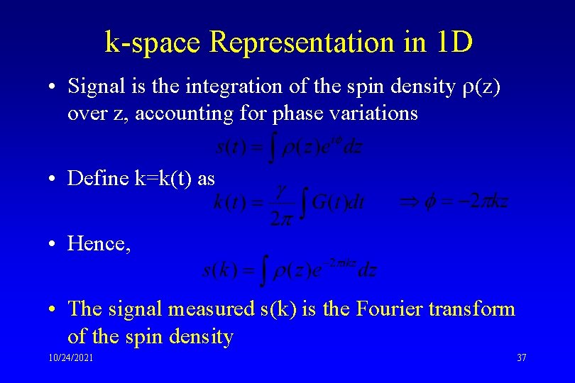
k-space Representation in 1 D • Signal is the integration of the spin density (z) over z, accounting for phase variations • Define k=k(t) as • Hence, • The signal measured s(k) is the Fourier transform of the spin density 10/24/2021 37

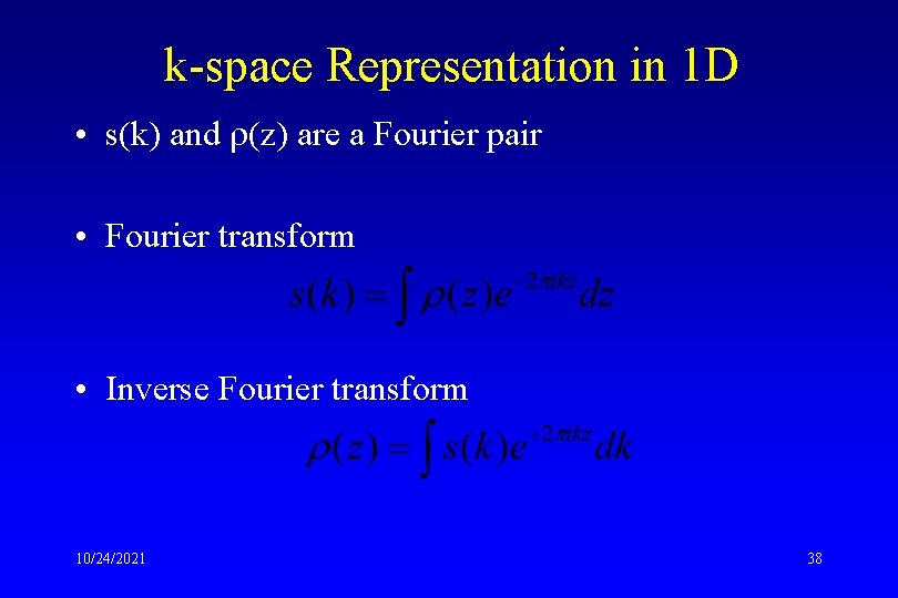
k-space Representation in 1 D • s(k) and (z) are a Fourier pair • Fourier transform • Inverse Fourier transform 10/24/2021 38

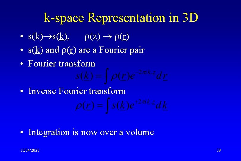
k-space Representation in 3 D • s(k), (z) (r) • s(k) and (r) are a Fourier pair • Fourier transform • Inverse Fourier transform • Integration is now over a volume 10/24/2021 39

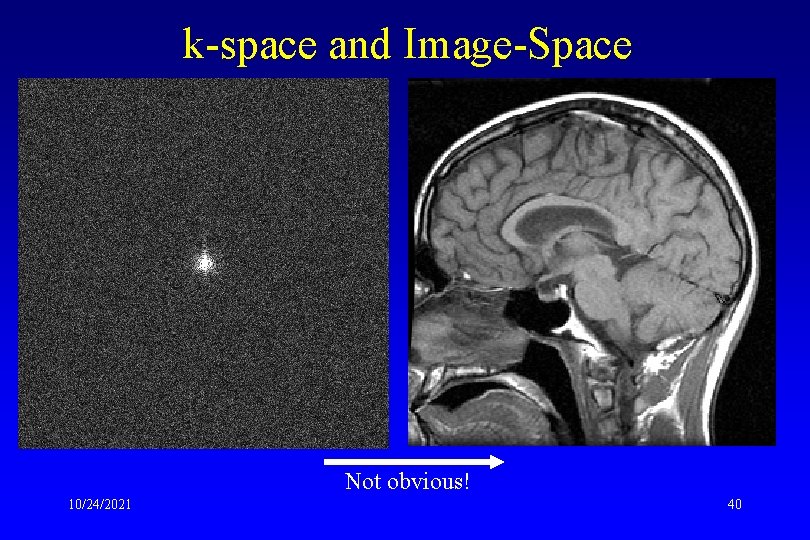
k-space and Image-Space Not obvious! 10/24/2021 40