Longrange correlations in driven systems David Mukamel Driven

Long-range correlations in driven systems David Mukamel

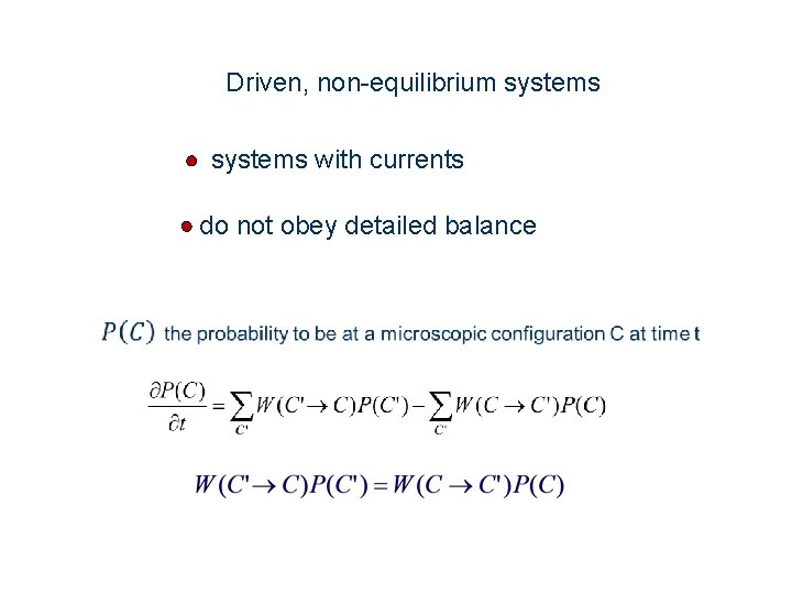
Driven, non-equilibrium systems with currents do not obey detailed balance

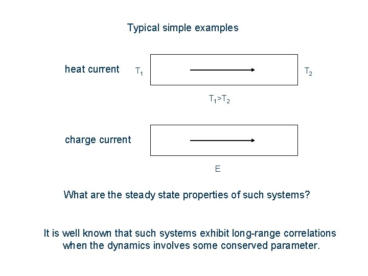
Typical simple examples heat current T 1 T 2 T 1>T 2 charge current E What are the steady state properties of such systems? It is well known that such systems exhibit long-range correlations when the dynamics involves some conserved parameter.

Outline Will discuss a few examples where long-range correlations show up and consider some consequences Example I: Effect of a local drive on the steady state of a system Example II: Linear drive in two dimensions: spontaneous symmetry breaking

Example I : Local drive perturbation T. Sadhu, S. Majumdar, DM, Phys. Rev. E 84, 051136 (2011)

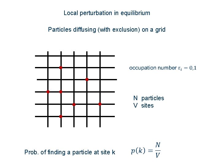
Local perturbation in equilibrium Particles diffusing (with exclusion) on a grid N particles V sites Prob. of finding a particle at site k

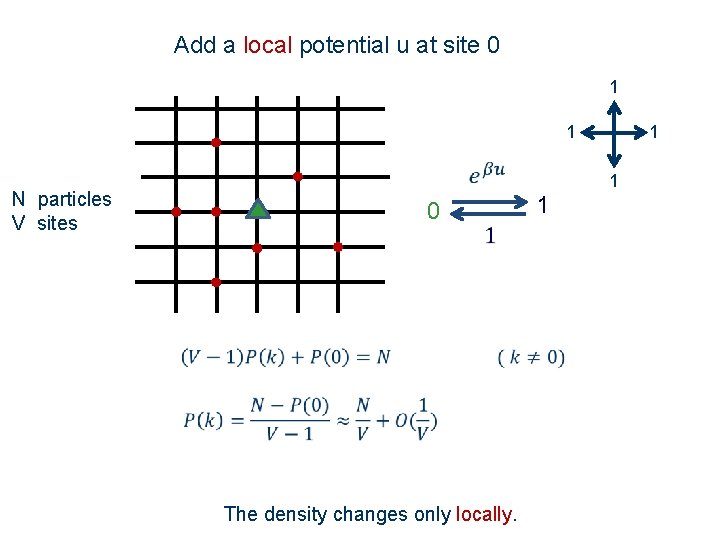
Add a local potential u at site 0 1 1 N particles V sites 0 1 1 The density changes only locally. 1

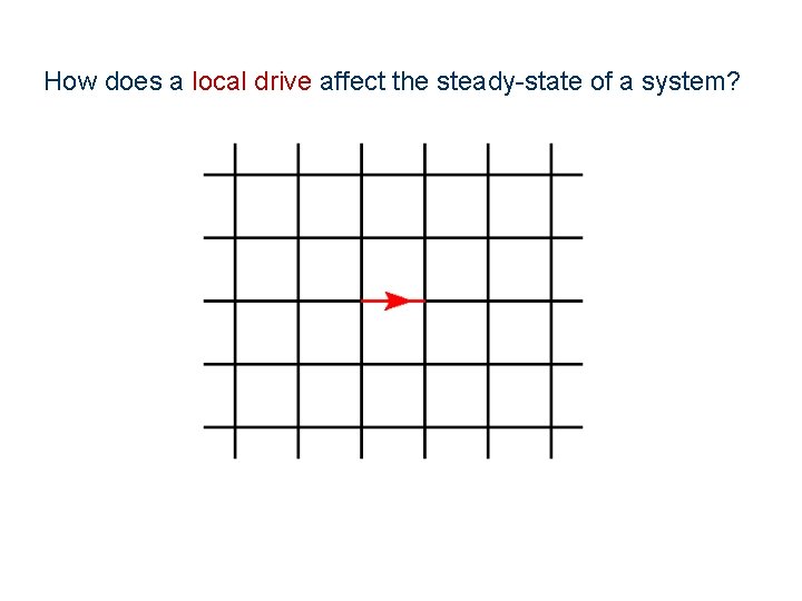
How does a local drive affect the steady-state of a system?

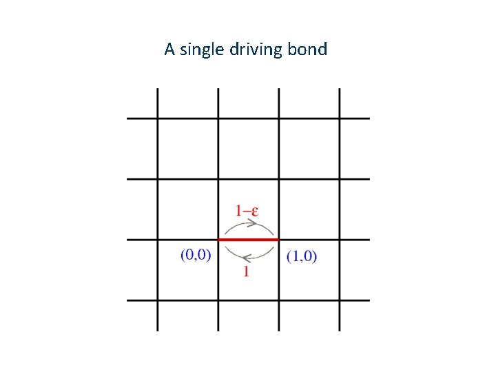
A single driving bond

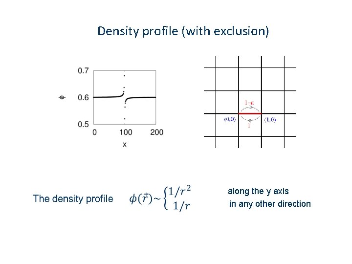
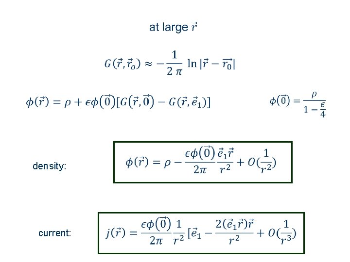
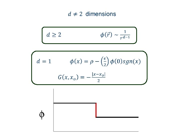
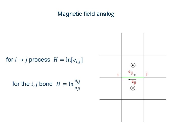
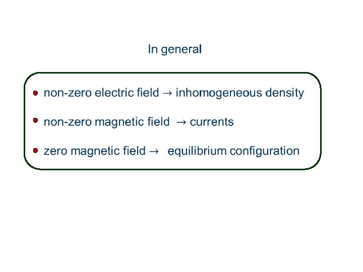
Main results: In d ≥ 2 dimensions both the density and the local current decay algebraically with the distance from the driven bond. The same is true for local arrangements of driven bond. The power law of the decay depends on the specific configuration. In d=2 dimensions a close correspondence to electrostatics is found, with analogous variables to electric and magnetic fields E, H.

Density profile (with exclusion) along the y axis in any other direction

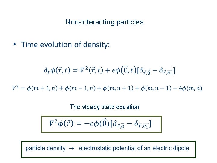
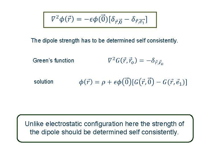
Non-interacting particles • The steady state equation

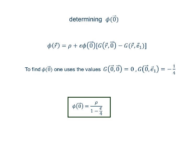
The dipole strength has to be determined self consistently. Green’s function solution Unlike electrostatic configuration here the strength of the dipole should be determined self consistently.

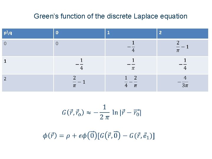
Green’s function of the discrete Laplace equation pq 0 0 0 1 2

density: current:

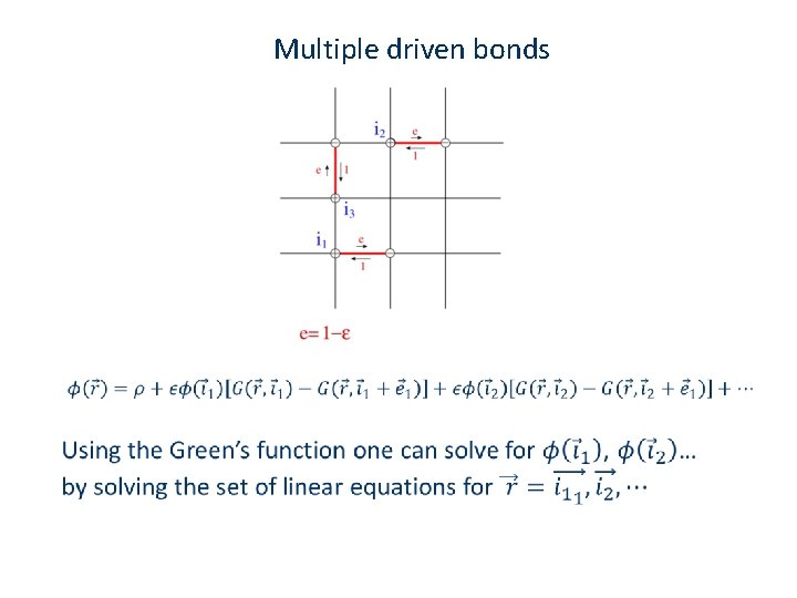
Multiple driven bonds

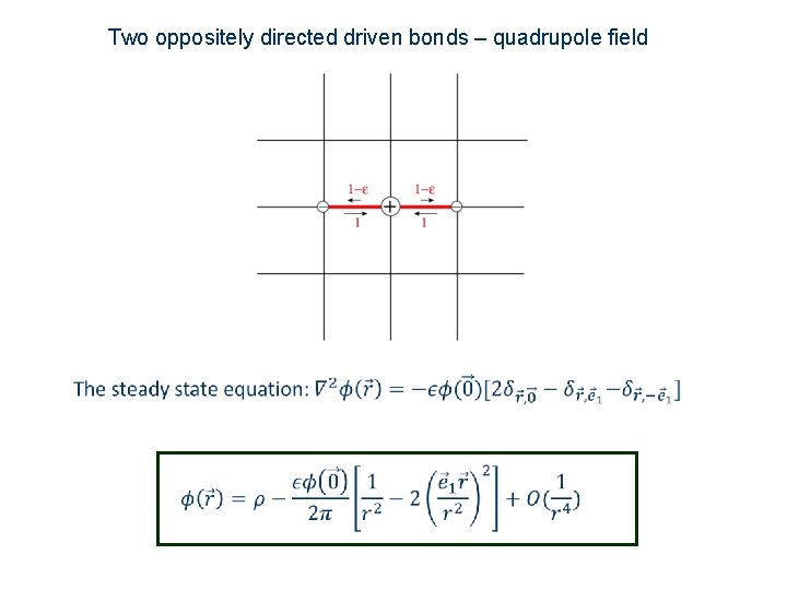
Two oppositely directed driven bonds – quadrupole field

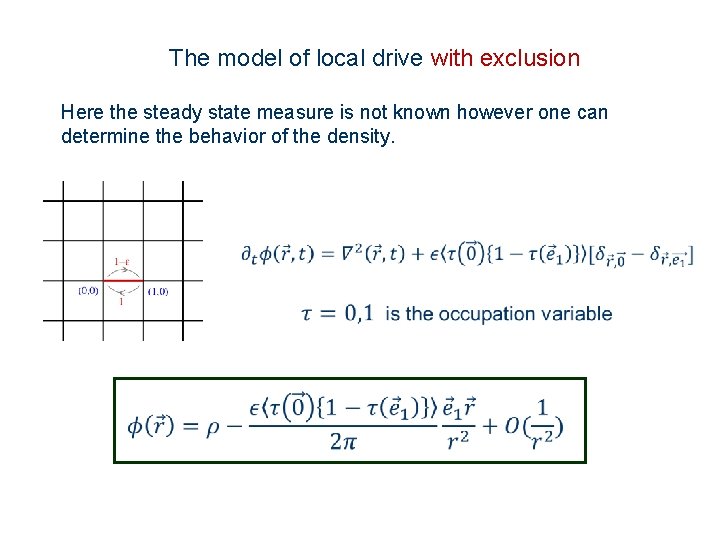
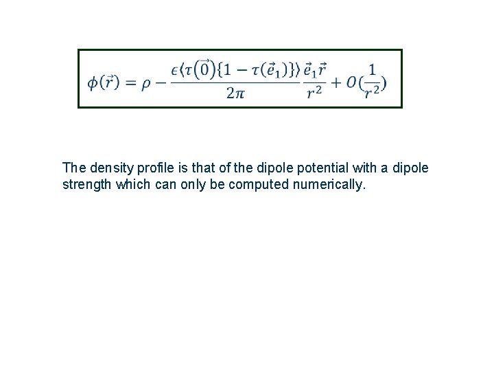
The model of local drive with exclusion Here the steady state measure is not known however one can determine the behavior of the density.

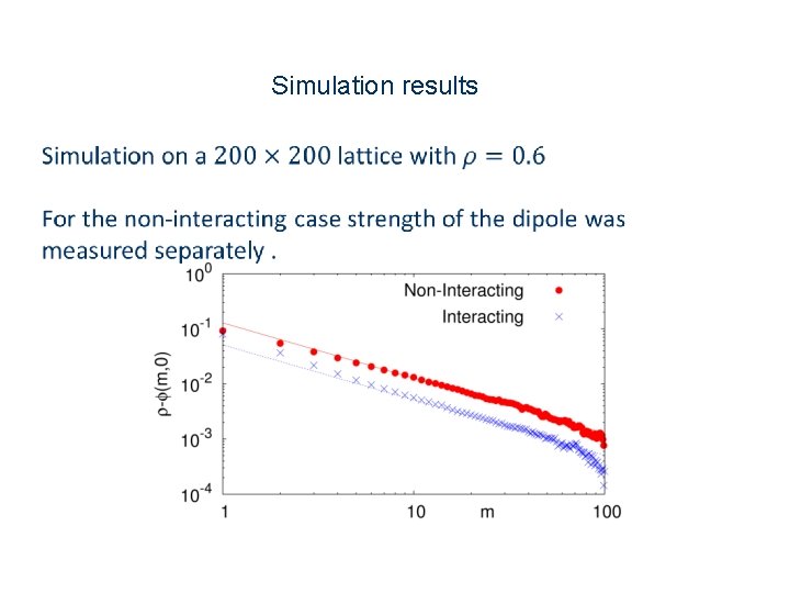
The density profile is that of the dipole potential with a dipole strength which can only be computed numerically.

Simulation results

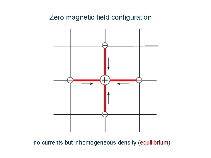
Magnetic field analog

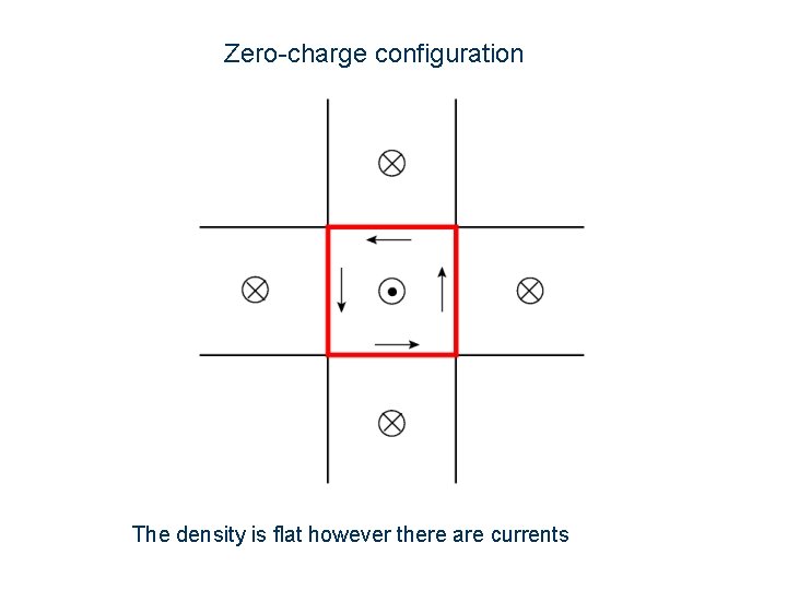
Zero-charge configuration The density is flat however there are currents

Zero magnetic field configuration no currents but inhomogeneous density (equilibrium)

Example II: a two dimensional model with a driven line T. Sadhu, Z. Shapira, DM

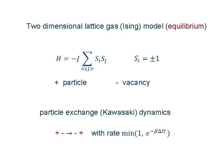
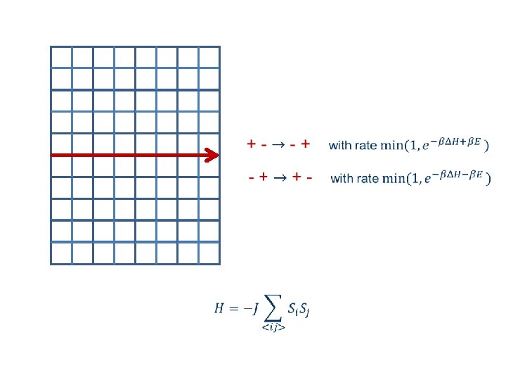
Two dimensional lattice gas (Ising) model (equilibrium) + particle - vacancy particle exchange (Kawasaki) dynamics

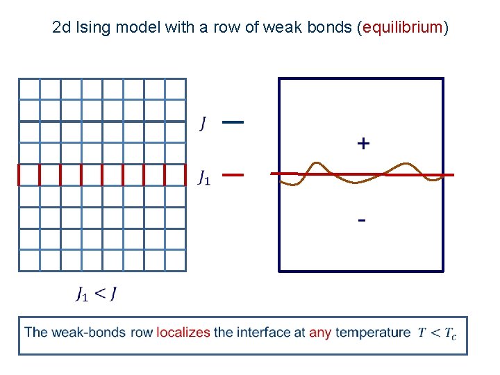
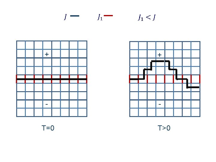
2 d Ising model with a row of weak bonds (equilibrium) +

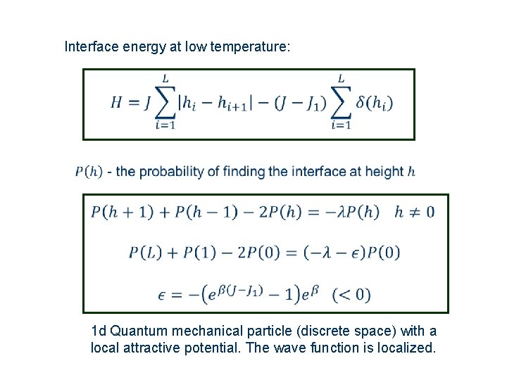
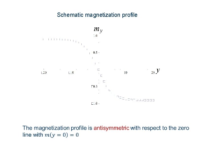
Interface energy at low temperature: 1 d Quantum mechanical particle (discrete space) with a local attractive potential. The wave function is localized.

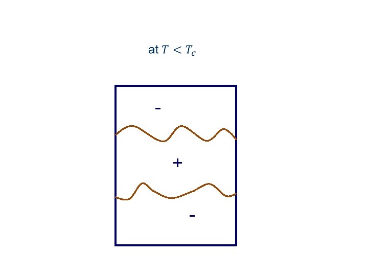
Schematic magnetization profile

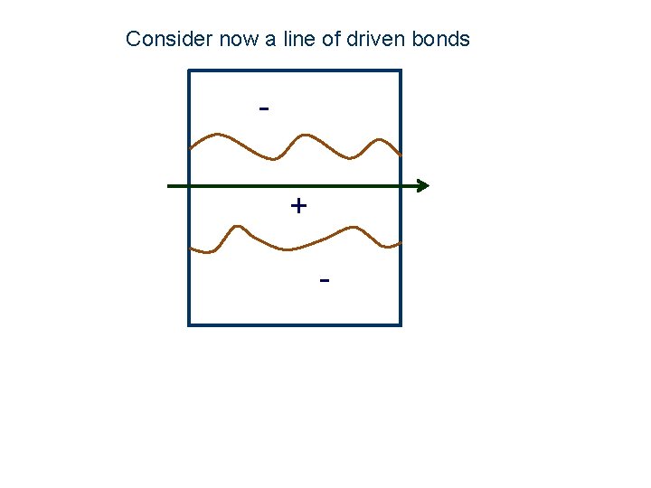
Consider now a line of driven bonds + -

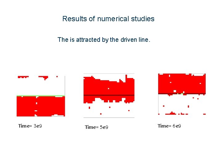
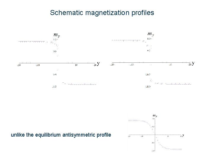
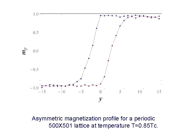
Main results The driven line attracts the interface The interface width is finite (localized) A spontaneous symmetry breaking takes place by which the magnetization of the driven line is non-zero and the magnetization profile is not antisymmetric, (mesoscopic transition). The fluctuation of the interface are not symmetric around the driven line. These results can be demonstrated analytically in certain limit.

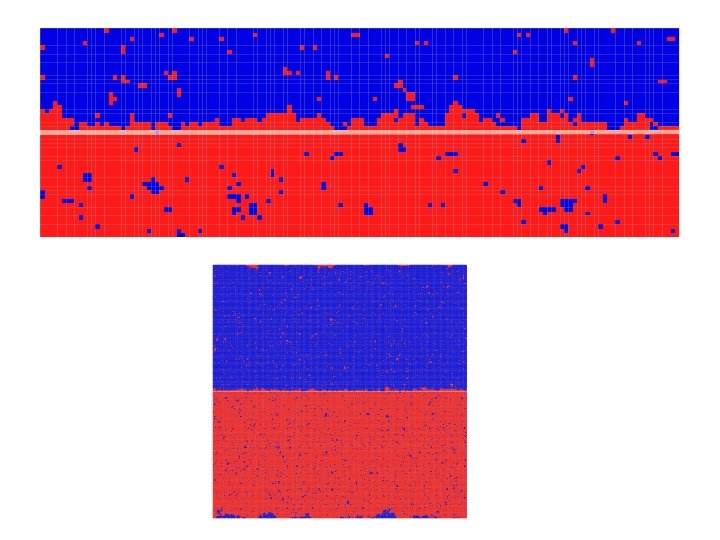
Results of numerical studies The is attracted by the driven line. Time= 3 e 9 Time= 5 e 9 Time= 6 e 9

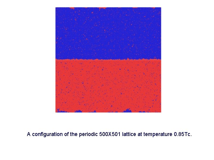
A configuration of the periodic 500 X 501 lattice at temperature 0. 85 Tc.

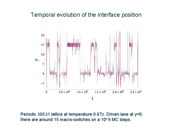
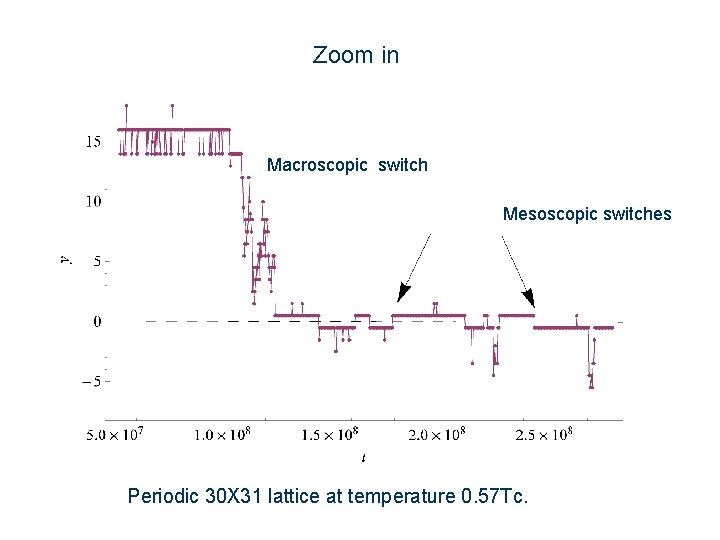
Temporal evolution of the interface position Periodic 30 X 31 lattice at temperature 0. 6 Tc. Driven lane at y=0, there around 15 macro-switches on a 10^9 MC steps.

Zoom in Macroscopic switch Mesoscopic switches Periodic 30 X 31 lattice at temperature 0. 57 Tc.

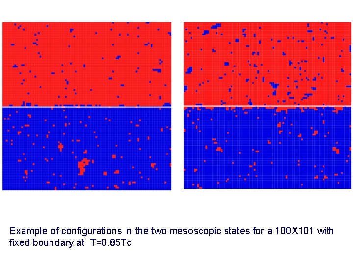
Example of configurations in the two mesoscopic states for a 100 X 101 with fixed boundary at T=0. 85 Tc

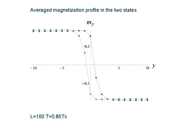
Schematic magnetization profiles unlike the equilibrium antisymmetric profile

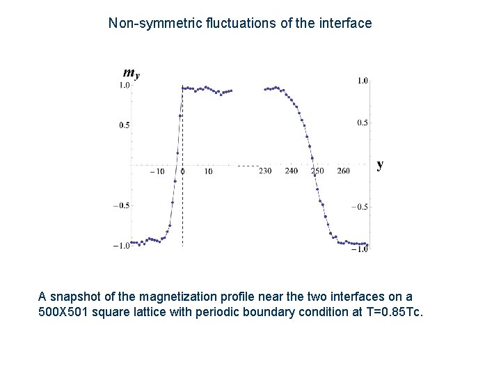
Asymmetric magnetization profile for a periodic 500 X 501 lattice at temperature T=0. 85 Tc.

Non-symmetric fluctuations of the interface A snapshot of the magnetization profile near the two interfaces on a 500 X 501 square lattice with periodic boundary condition at T=0. 85 Tc.

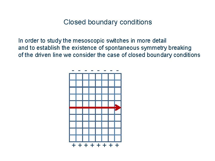
Closed boundary conditions In order to study the mesoscopic switches in more detail and to establish the existence of spontaneous symmetry breaking of the driven line we consider the case of closed boundary conditions - - - - + + + +

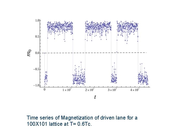
Time series of Magnetization of driven lane for a 100 X 101 lattice at T= 0. 6 Tc.

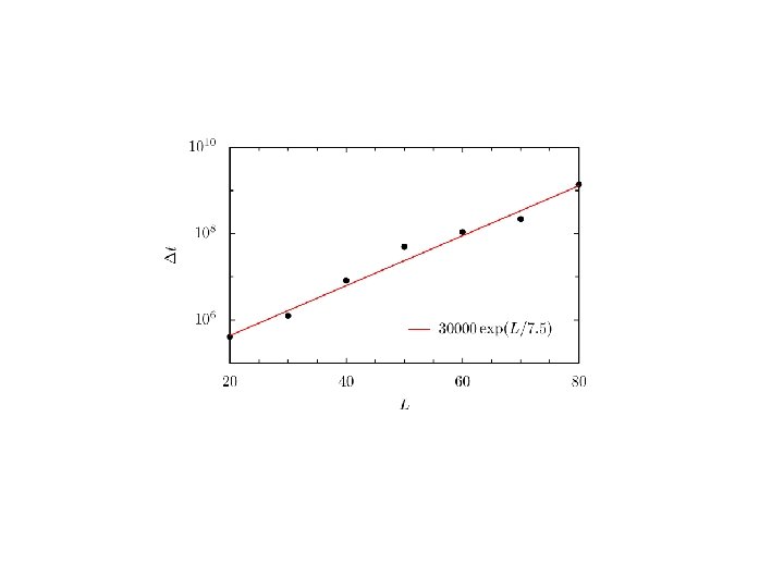
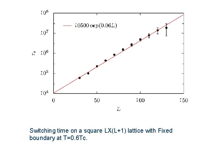
Switching time on a square LX(L+1) lattice with Fixed boundary at T=0. 6 Tc.

Averaged magnetization profile in the two states L=100 T=0. 85 Tc

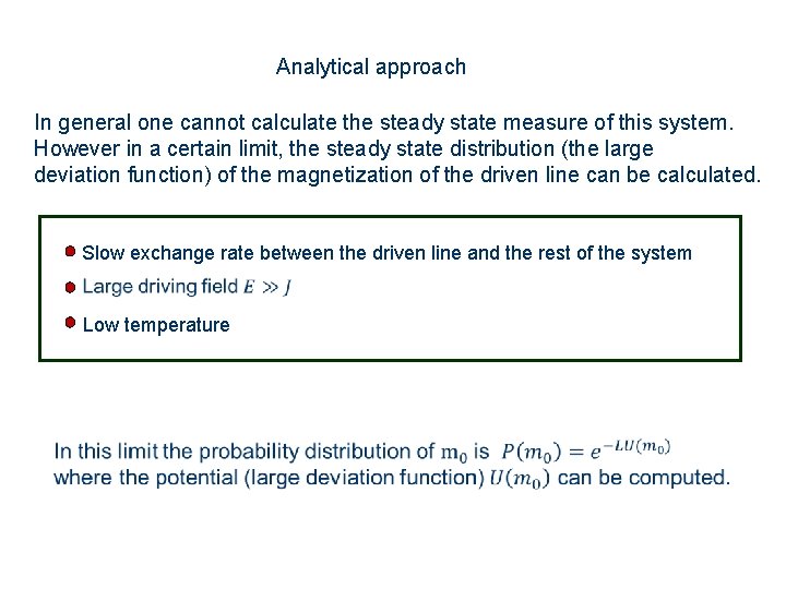
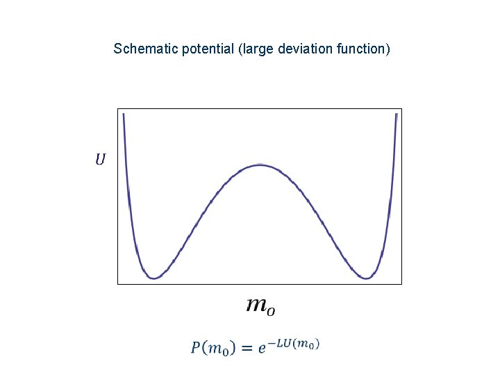
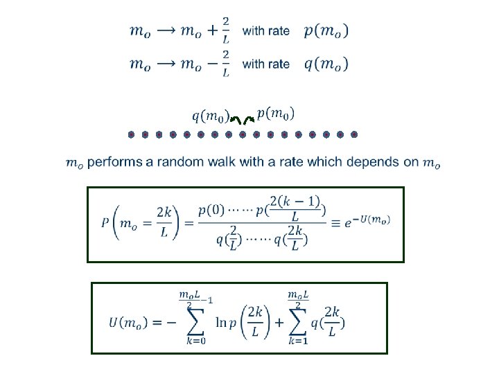
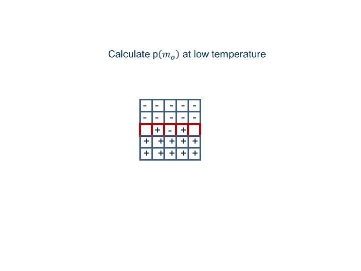
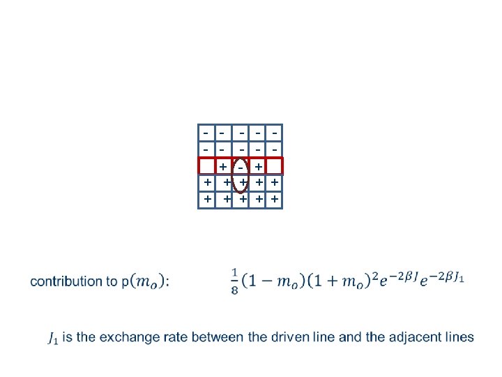
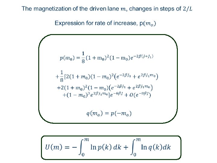
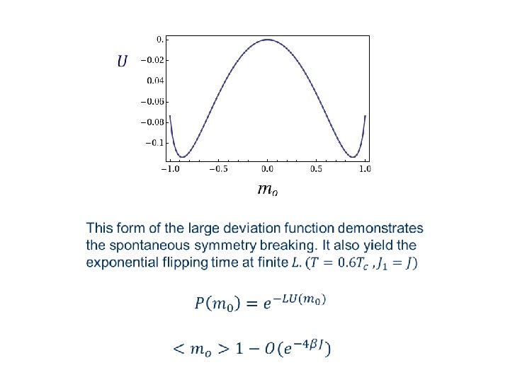
Analytical approach In general one cannot calculate the steady state measure of this system. However in a certain limit, the steady state distribution (the large deviation function) of the magnetization of the driven line can be calculated. Slow exchange rate between the driven line and the rest of the system Low temperature

Schematic potential (large deviation function)

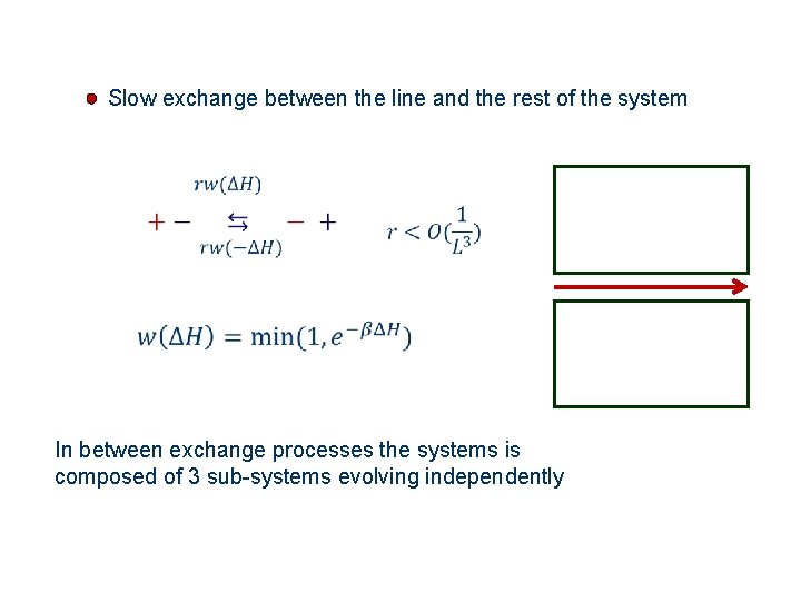
Slow exchange between the line and the rest of the system In between exchange processes the systems is composed of 3 sub-systems evolving independently

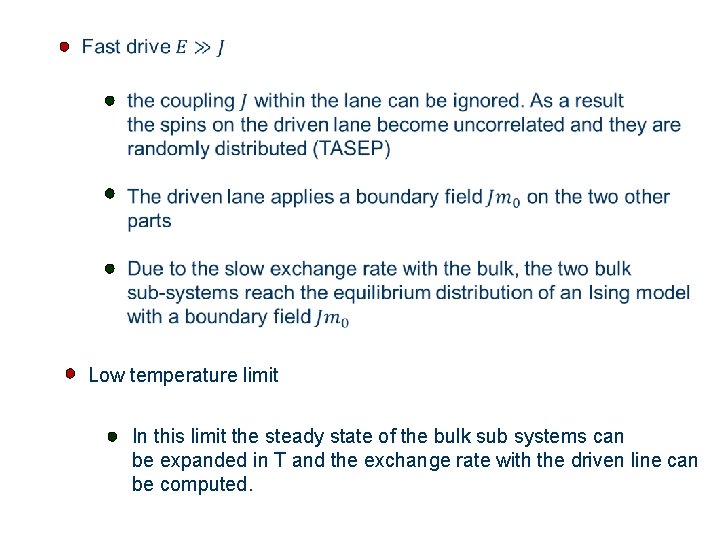
Low temperature limit In this limit the steady state of the bulk sub systems can be expanded in T and the exchange rate with the driven line can be computed.

Summary Driven systems exhibit long range correlations under generic conditions. Such correlations sometimes lead to long-range order and spontaneous symmetry breaking which are absent under equilibrium conditions. Simple examples of these phenomena have been presented. A limit of slow exchange rate is discussed which enables the evaluation of some large deviation functions far from equilibrium.