Local Computations in LargeScale Networks Idit Keidar Technion

Local Computations in Large-Scale Networks Idit Keidar Technion

Material I. Keidar and A. Schuster: “Want Scalable Computing? Speculate!” SIGACT News Sep 2006. http: //www. ee. technion. ac. il/people/idish/ftp/speculate. pdf Y. Birk, I. Keidar, L. Liss, A. Schuster, and R. Wolff: “Veracity Radius - Capturing the Locality of Distributed Computations”. PODC'06. http: //www. ee. technion. ac. il/people/idish/ftp/veracity_radius. pdf Y. Birk, I. Keidar, L. Liss, and A. Schuster: “Efficient Dynamic Aggregation”. DISC'06. http: //www. ee. technion. ac. il/people/idish/ftp/eff_dyn_agg. pdf E. Bortnikov, I. Cidon and I. Keidar: “Scalable Load-Distance Balancing in Large Networks”. DISC’ 07. http: //www. ee. technion. ac. il/people/idish/ftp/LD-Balancing. pdf

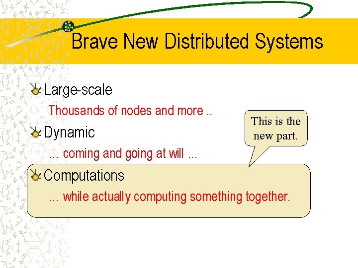
Brave New Distributed Systems Large-scale Thousands of nodes and more. . Dynamic This is the new part. … coming and going at will. . . Computations … while actually computing something together.

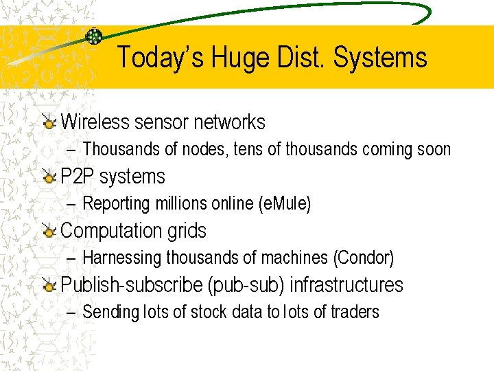
Today’s Huge Dist. Systems Wireless sensor networks – Thousands of nodes, tens of thousands coming soon P 2 P systems – Reporting millions online (e. Mule) Computation grids – Harnessing thousands of machines (Condor) Publish-subscribe (pub-sub) infrastructures – Sending lots of stock data to lots of traders

Not Computing Together Yet Wireless sensor networks – Typically disseminate information to central location P 2 P & pub-sub systems – Simple file sharing, content distribution – Topology does not adapt to global considerations – Offline optimizations (e. g. , clustering) Computation grids – “Embarrassingly parallel” computations

Emerging Dist. Systems – Examples Autonomous sensor networks – Computations inside the network, e. g. , detecting trouble Wireless mesh network (WMN) management – Topology control – Assignment of users to gateways Adapting p 2 p overlays based on global considerations Data grids (information retrieval)

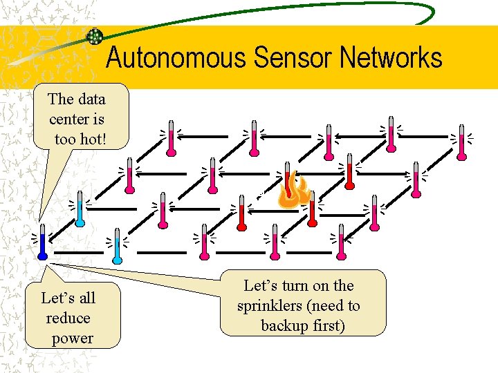
Autonomous Sensor Networks The data center is too hot! Let’s all reduce power Let’s turn on the sprinklers (need to backup first)

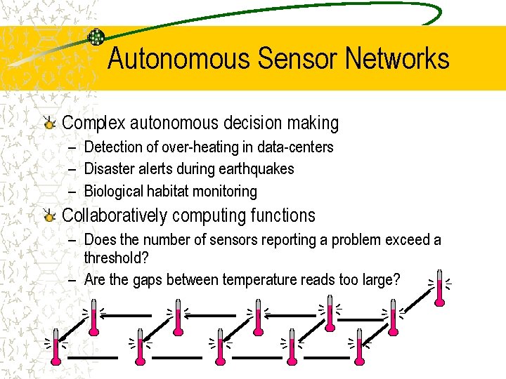
Autonomous Sensor Networks Complex autonomous decision making – Detection of over-heating in data-centers – Disaster alerts during earthquakes – Biological habitat monitoring Collaboratively computing functions – Does the number of sensors reporting a problem exceed a threshold? – Are the gaps between temperature reads too large?

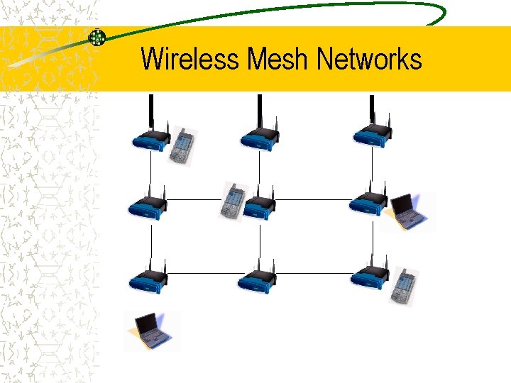
Wireless Mesh Networks

Wireless Mesh Networks Infrastructure (unlike MANET) City-wide coverage Supports wireless devices Connections to Mesh and out to the Internet – “The last mile” Cheap – Commodity wireless routers (hot spots) – Few Internet connections

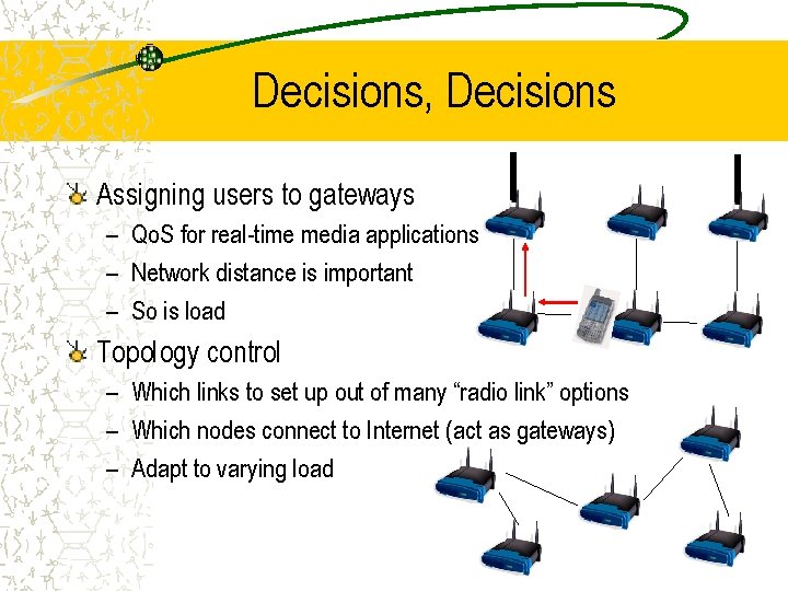
Decisions, Decisions Assigning users to gateways – Qo. S for real-time media applications – Network distance is important – So is load Topology control – Which links to set up out of many “radio link” options – Which nodes connect to Internet (act as gateways) – Adapt to varying load

Centralized Solutions Don’t Cut It Load Communication costs Delays Fault-tolerance

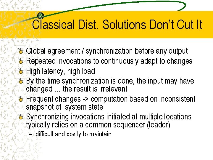
Classical Dist. Solutions Don’t Cut It Global agreement / synchronization before any output Repeated invocations to continuously adapt to changes High latency, high load By the time synchronization is done, the input may have changed … the result is irrelevant Frequent changes -> computation based on inconsistent snapshot of system state Synchronizing invocations initiated at multiple locations typically relies on a common sequencer (leader) – difficult and costly to maintain

Locality to the Rescue! Nodes make local decisions based on communication (or synchronization) with some proximate nodes, rather than the entire network Infinitely scalable Fast, low overhead, low power, … L

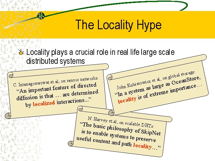
The Locality Hype Locality plays a crucial role in real life large scale distributed systems et. al, on sensor t a iw w n o g a n C. Inta re, o t S n a Oce s bi a u e K g n r nce… la a Joh t s r a o p m e im yste s m a e r t n I x “ of e s i y t i local networks: l, o z et. a atowic ected ir d f o e r tu a e f t “An importan rmined te e d e r a … t a diffusion is th actions. . . ” r te in d e z li a c by lo N. Harvey rage: al sto n glob et “The basic. al, on scalable DHTs: philosophy of Skip. Net is to enabl e systems to useful con tent and pa preserve th locality …”

What is Locality? Worst case view – O(1) in problem size [Naor & Stockmeyer, 1993] – Less than the graph diameter [Linial, 1992] – Often applicable only to simplistic problems or approximations Average case view – Requires an a priori distribution of the inputs To be continued…

Interesting Problems Have Inherently Global Instances WMN gateway assignment: arbitrarily high load near one gateway – Need to offload as far as the end of the network Percentage of nodes whose input exceeds threshold in sensor networks: near-tie situation – All “votes” need to be counted Fortunately, they don’t happen too often

Speculation is the Key to Locality We want solutions to be “as local as possible” WMN gateway assignment example: – Fast decision and quiescence under even load – Computation time and communication adaptive to distance to which we need to offload A node cannot locally know whether the problem instance is local – Load may be at other end of the network Can speculate that it is (optimism )

Computations are Never “Done” Speculative output may be over-ruled Good for ever-changing inputs – Sensor readings, user loads, … Computing ever-changing outputs – User never knows if output will change • due to bad speculation or unreflected input change – Reflecting changes faster is better If input changes cease, output will eventually be correct – With speculation same as without

Summary: Prerequisites for Speculation Global synchronization is prohibitive Many instances amenable to local solutions Eventual correctness acceptable – No meaningful notion of a “correct answer” at every point in time – When the system stabilizes for “long enough”, the output should converge to the correct one

The Challenge: Find a Meaningful Notion for Locality Many real world problems are trivially global in the worst case Yet, practical algorithms have been shown to be local most of the time ! The challenge: find a theoretical metric that captures this empirical behavior

Reminder: Naïve Locality Definitions Worst case view – Often applicable only to simplistic problems or approximations Average case view – Requires an a priori distribution of the inputs

Instance-Locality Formal instance-based locality: – Local fault mending [Kutten, Peleg 95, Kutten, Patt-Shamir 97] – Growth-restricted graphs [Kuhn, Moscibroda, Wattenhofer 05] – MST [Elkin 04] Empirical locality: voting in sensor networks – Although some instances require global computation, most can stabilize (and become quiescent) locally – In small neighborhood, independent of graph size – [Wolff, Schuster 03, Liss, Birk, Wolf, Schuster 04]

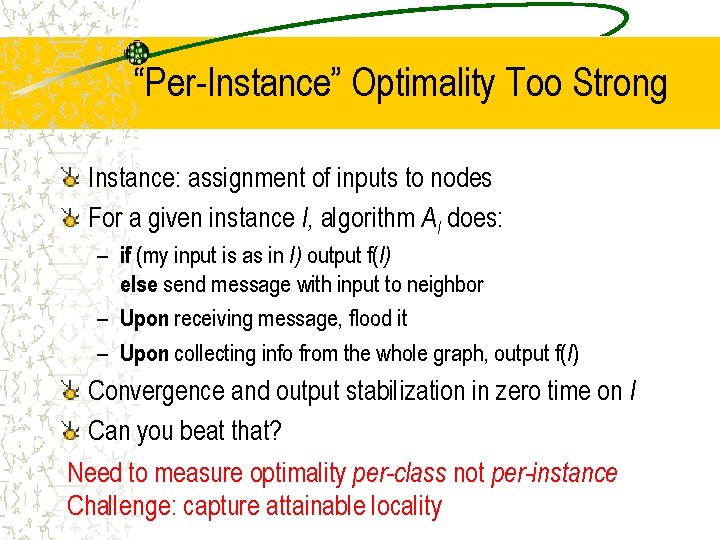
“Per-Instance” Optimality Too Strong Instance: assignment of inputs to nodes For a given instance I, algorithm AI does: – if (my input is as in I) output f(I) else send message with input to neighbor – Upon receiving message, flood it – Upon collecting info from the whole graph, output f(I) Convergence and output stabilization in zero time on I Can you beat that? Need to measure optimality per-class not per-instance Challenge: capture attainable locality

Local Complexity [BKLSW’ 06] Let – – – G be a family of graphs P be a problem on G M be a performance measure Classification CG of inputs to P on a graph G into classes C For class of inputs C, MLB(C) be a lower bound for computing P on all inputs in C Locality: G G C CG I C : MA(I) const MLB(C) A lower bound on a single instance is meaningless!

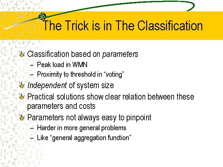
The Trick is in The Classification based on parameters – Peak load in WMN – Proximity to threshold in “voting” Independent of system size Practical solutions show clear relation between these parameters and costs Parameters not always easy to pinpoint – Harder in more general problems – Like “general aggregation function”

Veracity Radius – Capturing the Locality of Distributed Computations Yitzhak Birk, Idit Keidar, Liran Liss, Assaf Schuster, and Ran Wolf

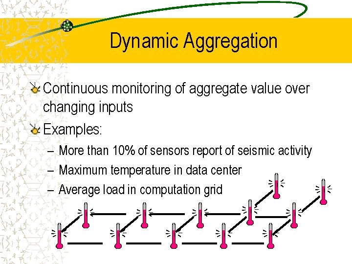
Dynamic Aggregation Continuous monitoring of aggregate value over changing inputs Examples: – More than 10% of sensors report of seismic activity – Maximum temperature in data center – Average load in computation grid

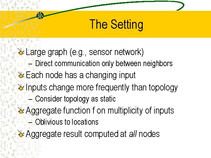
The Setting Large graph (e. g. , sensor network) – Direct communication only between neighbors Each node has a changing input Inputs change more frequently than topology – Consider topology as static Aggregate function f on multiplicity of inputs – Oblivious to locations Aggregate result computed at all nodes

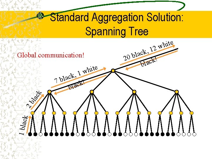
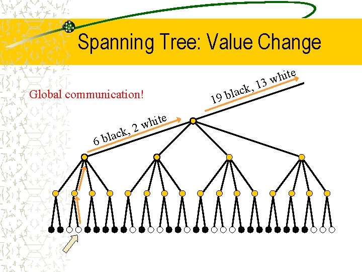
Goals for Dynamic Aggregation Fast convergence – If from some time t onward inputs do not change … • Output stabilization time from t • Quiescence time from t • Note: nodes do not know when stabilization and quiescence are achieved – If after stabilization input changes abruptly… Efficient communication – Zero communication when there are zero changes – Small changes little communication

Standard Aggregation Solution: Spanning Tree e it h w 12 Global communication! e 1 blac k 2 b lac k it h w 1 , k c 7 bla ck! bla k, c a l 20 b k! c a l b

Spanning Tree: Value Change e Global communication! k, c a l 6 b e t i h 2 w 1 ck a l b 9 , it h w 13

The Bad News Virtually every aggregation function has instances that cannot be computed without communicating with the whole graph – E. g. , majority voting when close to the threshold “every vote counts” Worst case analysis: convergence, quiescence times are (diameter)

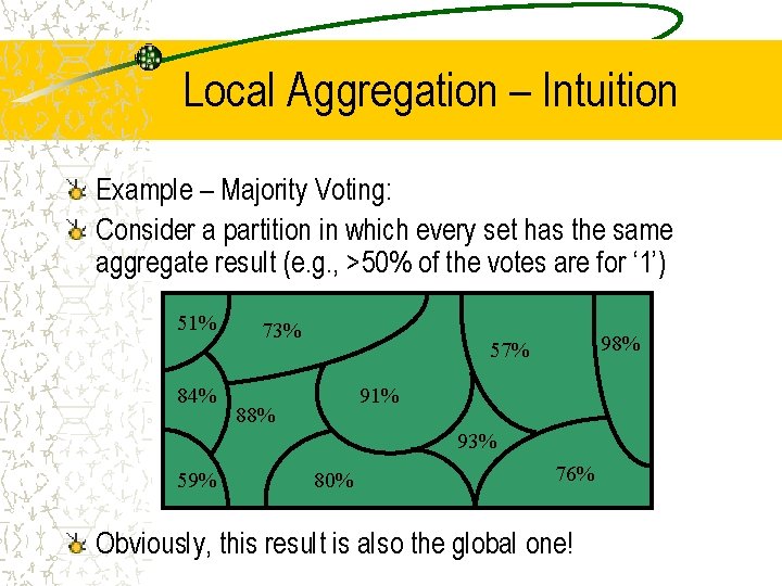
Local Aggregation – Intuition Example – Majority Voting: Consider a partition in which every set has the same aggregate result (e. g. , >50% of the votes are for ‘ 1’) 51% 84% 73% 98% 57% 91% 88% 93% 59% 80% 76% Obviously, this result is also the global one!

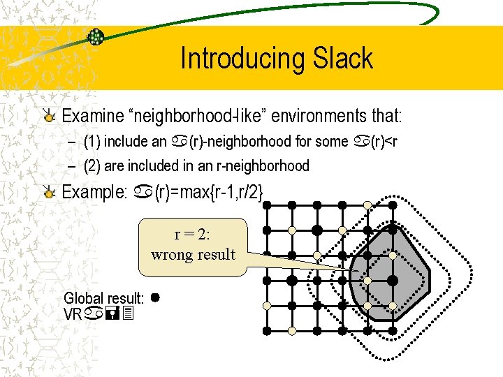
Veracity Radius (VR) for One-Shot Aggregation [BKLSW, PODC’ 06] Roughly speaking: the min radius r 0 such that "r> r 0: all r-neighborhoodshave same result Example: majority Radius 1: wrong result Radius 2: correct result VR=2

Introducing Slack Examine “neighborhood-like” environments that: – (1) include an a(r)-neighborhood for some a(r)<r – (2) are included in an r-neighborhood Example: a(r)=max{r-1, r/2} r = 2: wrong result Global result: VRa=3

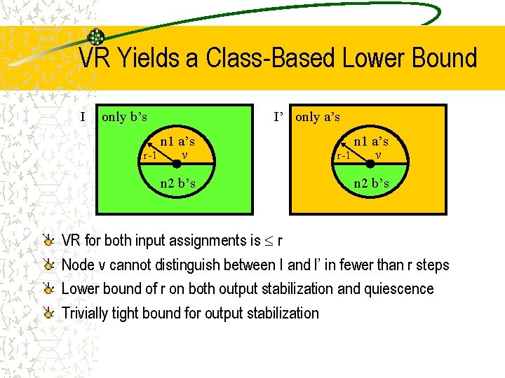
VR Yields a Class-Based Lower Bound I only b’s I’ only a’s n 1 a’s r-1 v n 2 b’s VR for both input assignments is r Node v cannot distinguish between I and I’ in fewer than r steps Lower bound of r on both output stabilization and quiescence Trivially tight bound for output stabilization

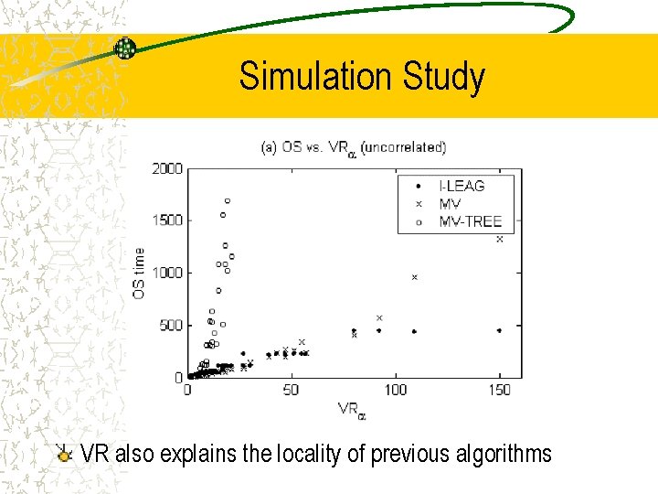
Veracity Radius Captures the Locality of One-Shot Aggregation [BKLSW, PODC’ 06] I-LEAG (Instance-Local Efficient Aggregation on Graphs) – Quiescence and output stabilization proportional to VR – Per-class within a factor of optimal – Local: depends on VR, not graph size! Note: nodes do not know VR or when stabilization and quiescence are achieved – Can’t expect to know you’re “done” in dynamic aggregation…

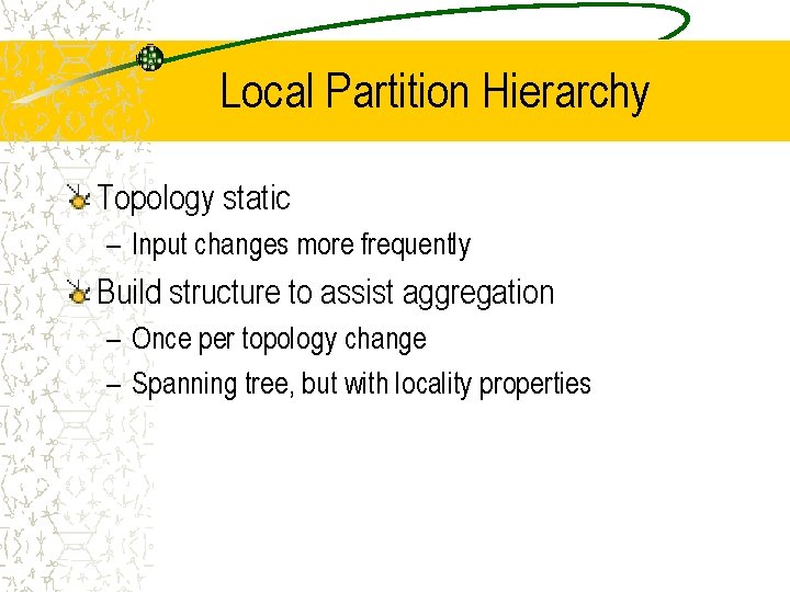
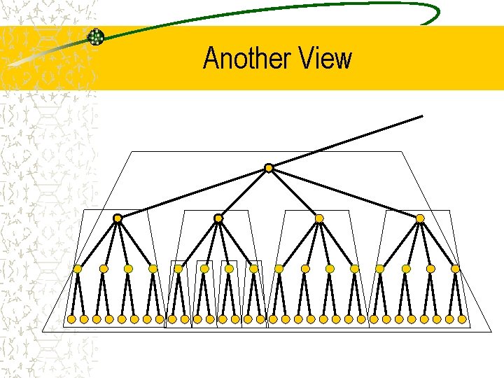
Local Partition Hierarchy Topology static – Input changes more frequently Build structure to assist aggregation – Once per topology change – Spanning tree, but with locality properties

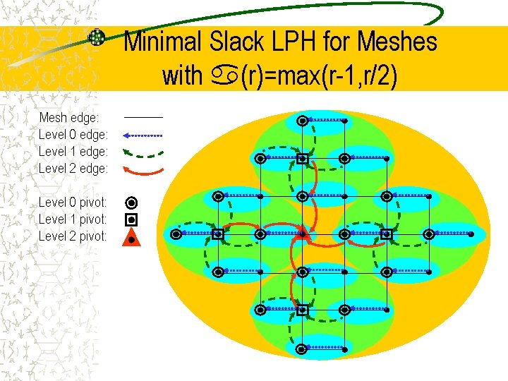
Minimal Slack LPH for Meshes with a(r)=max(r-1, r/2) Mesh edge: Level 0 edge: Level 1 edge: Level 2 edge: Level 0 pivot: Level 1 pivot: Level 2 pivot:

Another View

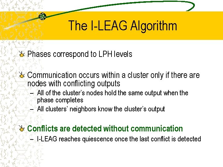
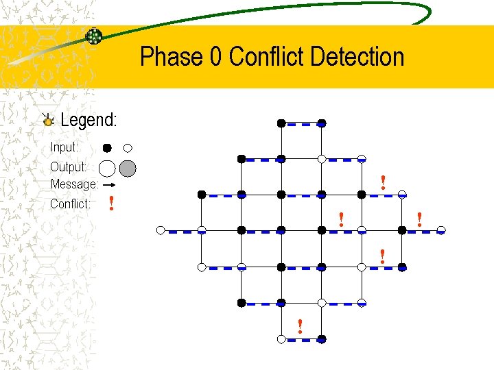
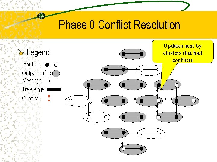
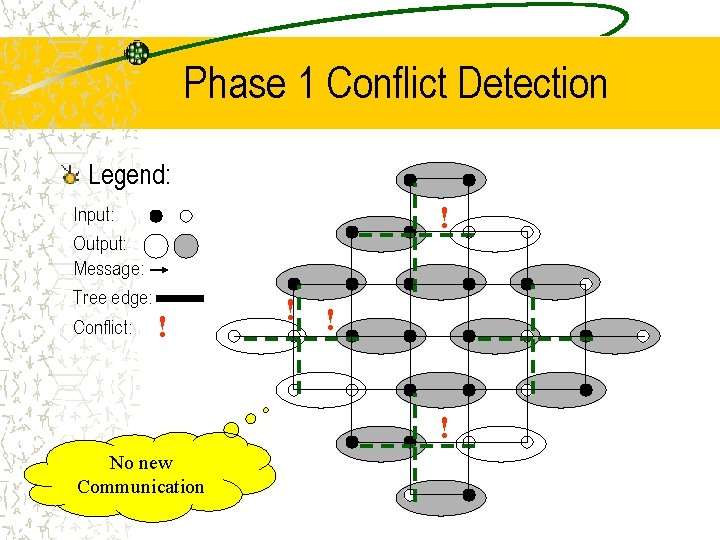
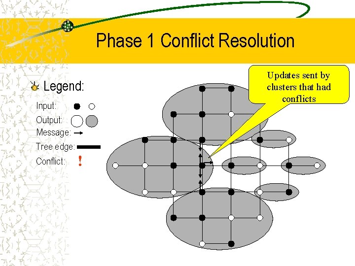
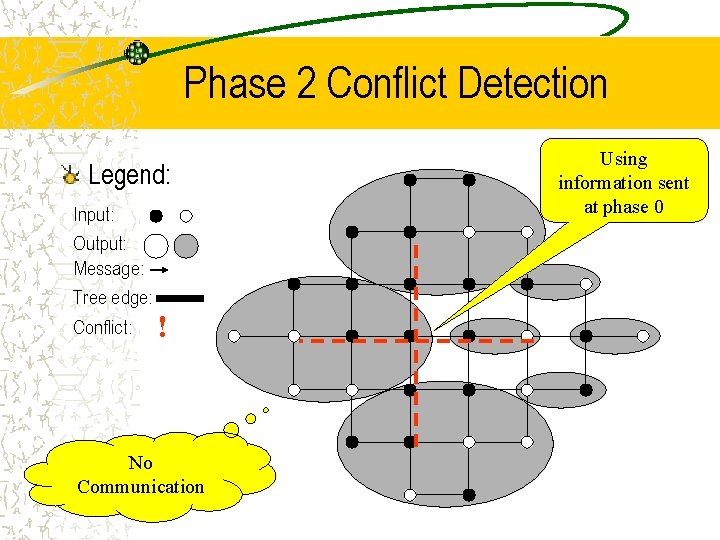
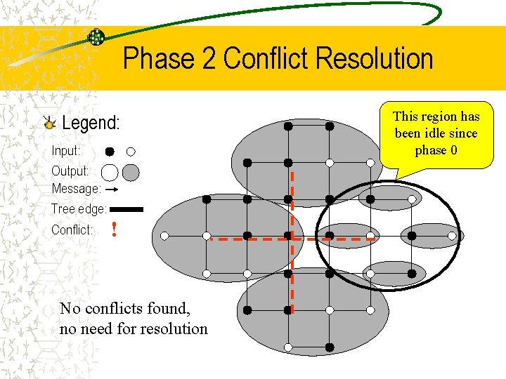
The I-LEAG Algorithm Phases correspond to LPH levels Communication occurs within a cluster only if there are nodes with conflicting outputs – All of the cluster’s nodes hold the same output when the phase completes – All clusters’ neighbors know the cluster’s output Conflicts are detected without communication – I-LEAG reaches quiescence once the last conflict is detected

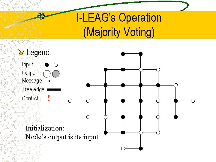
I-LEAG’s Operation (Majority Voting) Legend: Input: Output: Message: Tree edge: Conflict: ! Initialization: Node’s output is its input

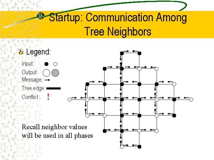
Startup: Communication Among Tree Neighbors Legend: Input: Output: Message: Tree edge: Conflict: ! Recall neighbor values will be used in all phases

Phase 0 Conflict Detection Legend: Input: Output: Message: Conflict: ! ! !

Phase 0 Conflict Resolution Legend: Input: Output: Message: Tree edge: Conflict: ! Updates sent by clusters that had conflicts

Phase 1 Conflict Detection Legend: Input: Output: Message: Tree edge: Conflict: ! ! ! No new Communication

Phase 1 Conflict Resolution Legend: Input: Output: Message: Tree edge: Conflict: ! Updates sent by clusters that had conflicts

Phase 2 Conflict Detection Legend: Input: Output: Message: Tree edge: Conflict: ! No Communication Using information sent at phase 0

Phase 2 Conflict Resolution Legend: Input: Output: Message: Tree edge: Conflict: ! No conflicts found, no need for resolution This region has been idle since phase 0

Simulation Study VR also explains the locality of previous algorithms

Efficient Dynamic Aggregation Yitzhak Birk, Idit Keidar, Liran Liss, and Assaf Schuster

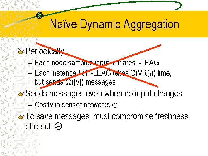
Naïve Dynamic Aggregation Periodically, – Each node samples input, initiates I-LEAG – Each instance I of I-LEAG takes O(VR(I)) time, but sends (|V|) messages Sends messages even when no input changes – Costly in sensor networks To save messages, must compromise freshness of result

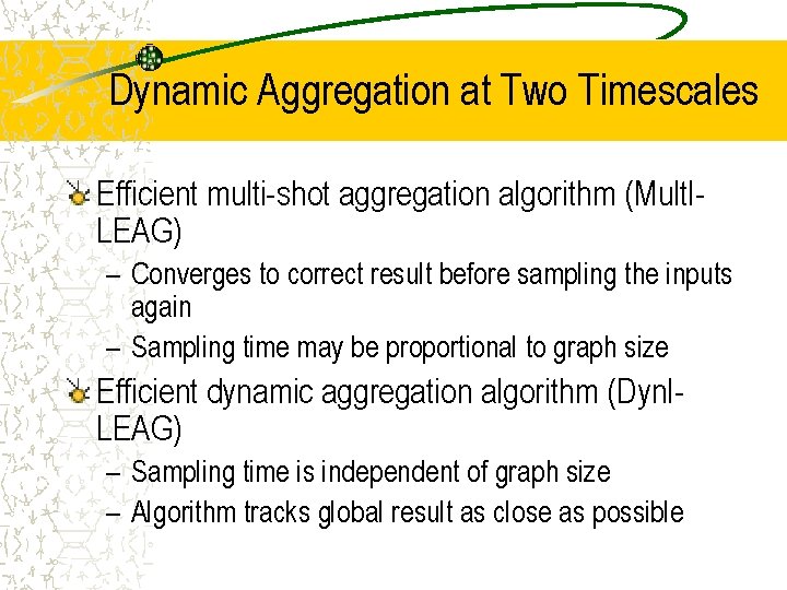
Dynamic Aggregation at Two Timescales Efficient multi-shot aggregation algorithm (Mult. ILEAG) – Converges to correct result before sampling the inputs again – Sampling time may be proportional to graph size Efficient dynamic aggregation algorithm (Dyn. ILEAG) – Sampling time is independent of graph size – Algorithm tracks global result as close as possible

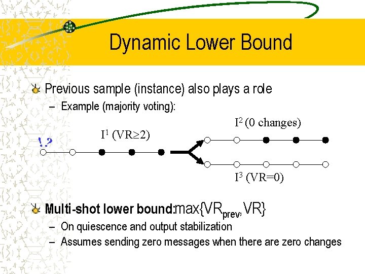
Dynamic Lower Bound Previous sample (instance) also plays a role – Example (majority voting): !? I 1 (VR 2) I 2 (0 changes) I 3 (VR=0) Multi-shot lower bound: max{VRprev, VR} – On quiescence and output stabilization – Assumes sending zero messages when there are zero changes

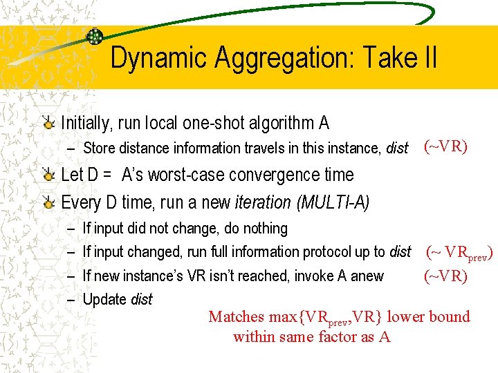
Dynamic Aggregation: Take II Initially, run local one-shot algorithm A – Store distance information travels in this instance, dist (~VR) Let D = A’s worst-case convergence time Every D time, run a new iteration (MULTI-A) – – If input did not change, do nothing If input changed, run full information protocol up to dist (~ VRprev) If new instance’s VR isn’t reached, invoke A anew (~VR) Update dist Matches max{VRprev, VR} lower bound within same factor as A

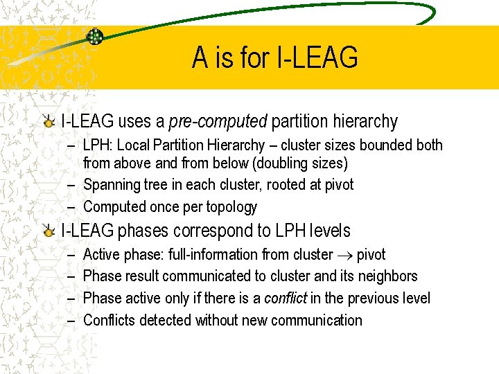
A is for I-LEAG uses a pre-computed partition hierarchy – LPH: Local Partition Hierarchy – cluster sizes bounded both from above and from below (doubling sizes) – Spanning tree in each cluster, rooted at pivot – Computed once per topology I-LEAG phases correspond to LPH levels – – Active phase: full-information from cluster pivot Phase result communicated to cluster and its neighbors Phase active only if there is a conflict in the previous level Conflicts detected without new communication

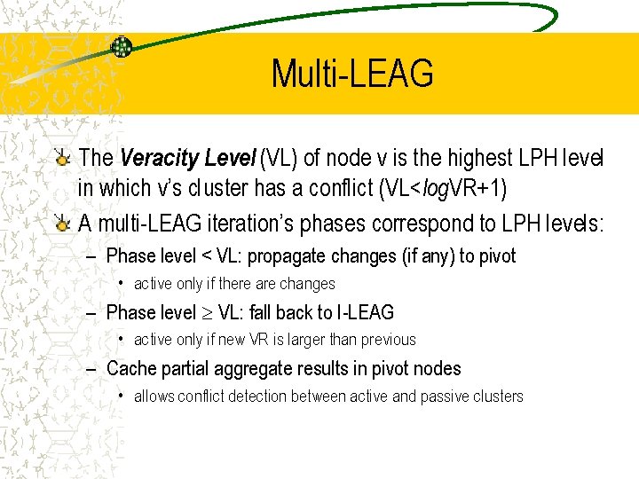
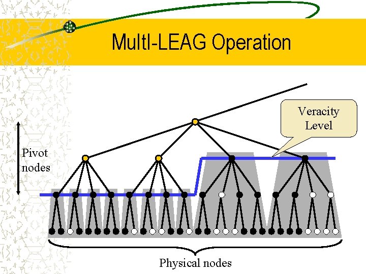
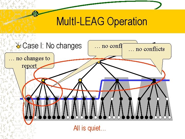
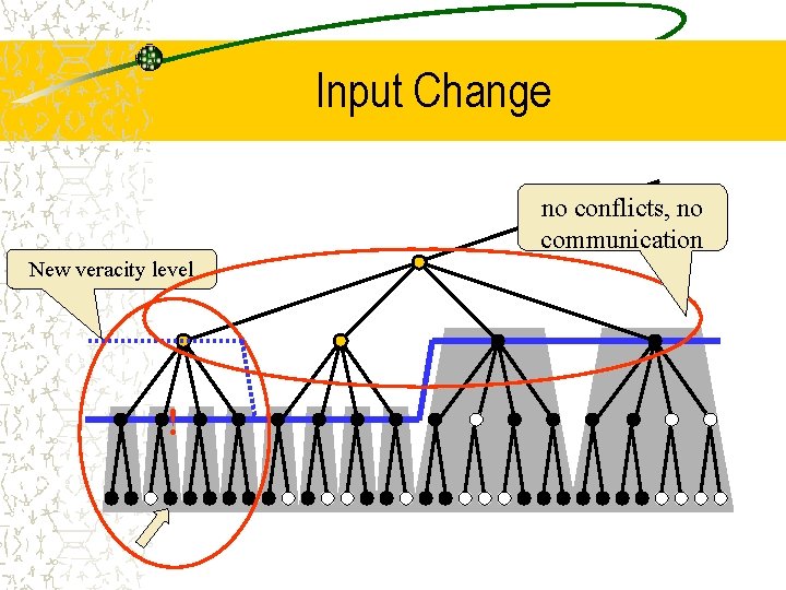
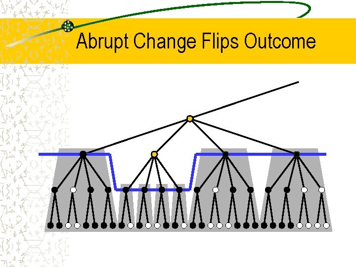
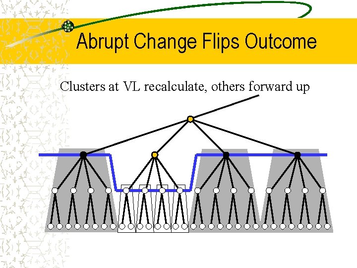
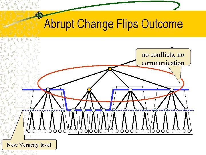
Multi-LEAG The Veracity Level (VL) of node v is the highest LPH level in which v’s cluster has a conflict (VL<log. VR+1) A multi-LEAG iteration’s phases correspond to LPH levels: – Phase level < VL: propagate changes (if any) to pivot • active only if there are changes – Phase level VL: fall back to I-LEAG • active only if new VR is larger than previous – Cache partial aggregate results in pivot nodes • allows conflict detection between active and passive clusters

Mult. I-LEAG Operation Veracity Level Pivot nodes Physical nodes

Mult. I-LEAG Operation Case I: No changes … no conflicts … no changes to report All is quiet…

Input Change no conflicts, no communication New veracity level !

Abrupt Change Flips Outcome

Abrupt Change Flips Outcome Clusters at VL recalculate, others forward up

Abrupt Change Flips Outcome no conflicts, no communication New Veracity level

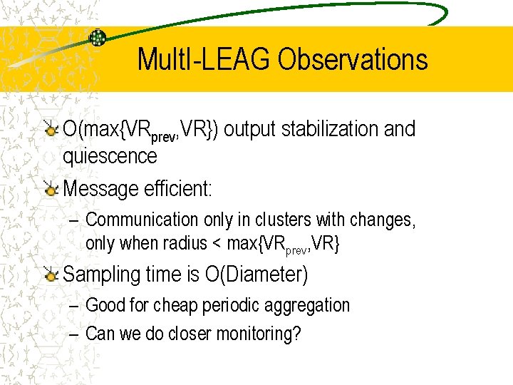
Mult. I-LEAG Observations O(max{VRprev, VR}) output stabilization and quiescence Message efficient: – Communication only in clusters with changes, only when radius < max{VRprev, VR} Sampling time is O(Diameter) – Good for cheap periodic aggregation – Can we do closer monitoring?

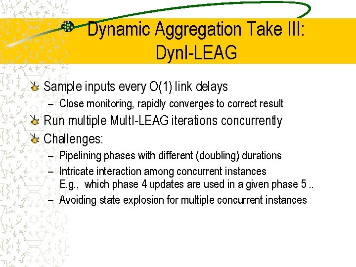
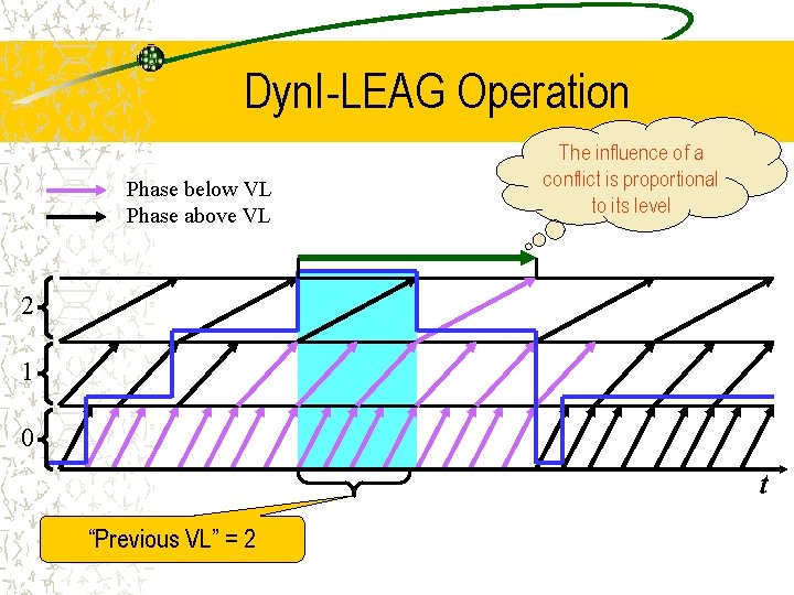
Dynamic Aggregation Take III: Dyn. I-LEAG Sample inputs every O(1) link delays – Close monitoring, rapidly converges to correct result Run multiple Mult. I-LEAG iterations concurrently Challenges: – Pipelining phases with different (doubling) durations – Intricate interaction among concurrent instances E. g. , which phase 4 updates are used in a given phase 5. . – Avoiding state explosion for multiple concurrent instances

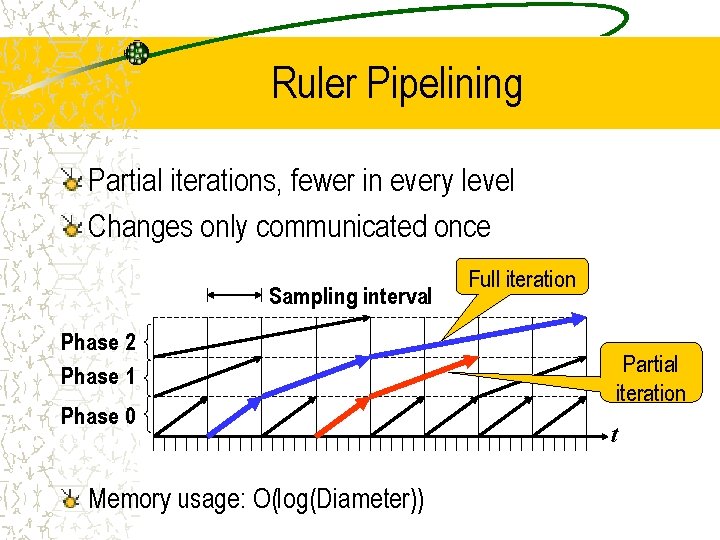
Ruler Pipelining Partial iterations, fewer in every level Changes only communicated once Sampling interval Phase 2 Phase 1 Phase 0 Memory usage: O(log(Diameter)) Full iteration Partial iteration t

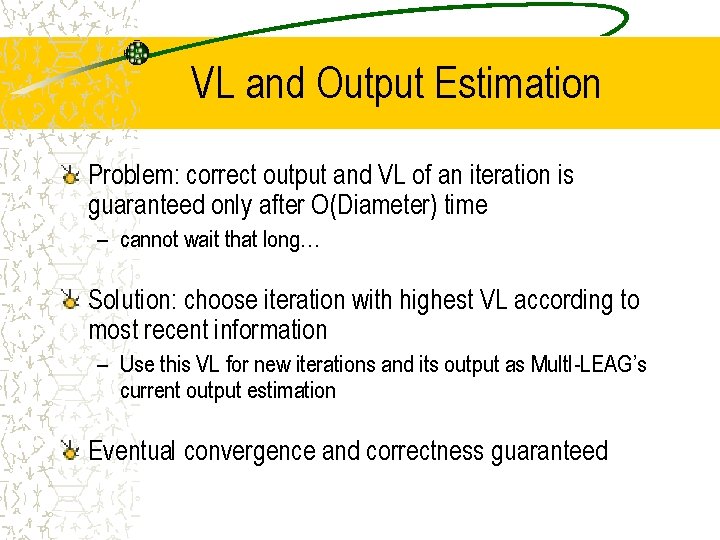
VL and Output Estimation Problem: correct output and VL of an iteration is guaranteed only after O(Diameter) time – cannot wait that long… Solution: choose iteration with highest VL according to most recent information – Use this VL for new iterations and its output as Mult. I-LEAG’s current output estimation Eventual convergence and correctness guaranteed

Dyn. I-LEAG Operation Phase below VL Phase above VL The influence of a conflict is proportional to its level 2 1 0 t “Previous VL” = 2

Dynamic Aggregation: Conclusions Local operation is possible – in dynamic systems – that solve inherently global problems Mult. I-LEAG delivers periodic correct snapshots at minimal cost Dyn. I-LEAG responds immediately to input changes with a slightly higher message rate

Scalable Load-Distance Balancing Edward Bortnikov, Israel Cidon, Idit Keidar

Load-Distance Balancing Two sources of service delay – Network delay (depends on distance to server) – Congestion delay (depends on server load) – Total = Network + Congestion Input – Network distances and congestion functions Optimization goal – Minimize the maximum total delay NP-complete, 2 -approximation exists

Distributed Setting Synchronous Distributed assignment computation – Initially, users report location to the closest servers – Servers communicate and compute the assignment Requirements: – Eventual quiescence – Eventual stability of assignment – Constant approximation of the optimal cost (parameter)

Impact of Locality Extreme global solution – Collect all data and compute assignment centrally – Guarantees optimal cost – Excessive communication/network latency Extreme local solution – Nearest-Server assignment – No communication – No approximation guarantee (can’t handle crowds) No “one-size-fits-all”?

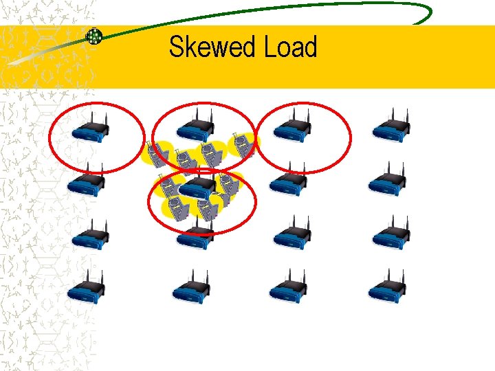
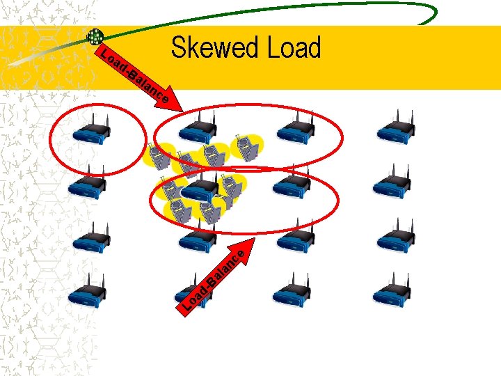
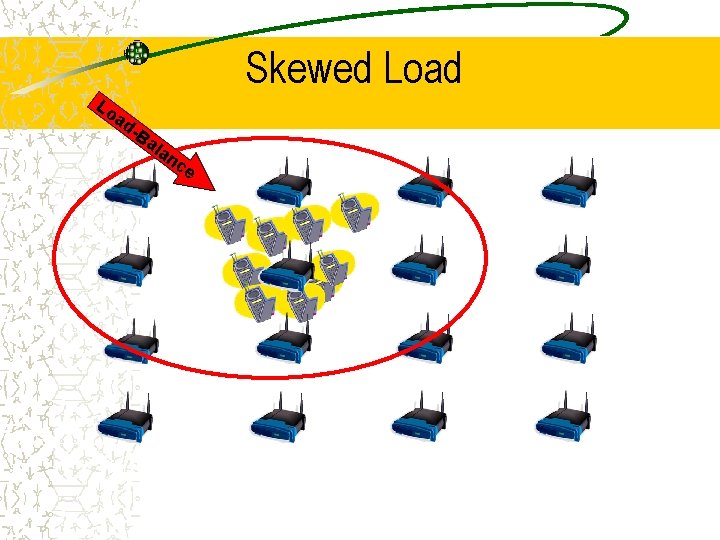
Workload-Sensitive Locality The cost function is distance-sensitive – Most assignments go to the near servers – … except for dissipating congestion peaks Key to distributed solution – Start from the Nearest-Server assignment – Load-balance congestion among near servers Communication locality is workload-sensitive – Go as far as needed … – … to achieve the required approximation

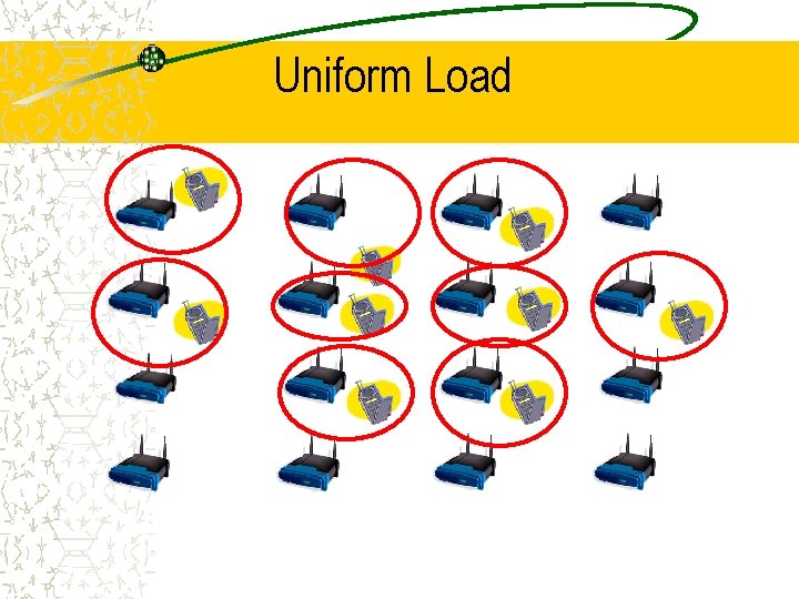
Uniform Load

Skewed Load

-B Skewed Load an c e al an ce ad -B al ad Lo Lo

Skewed Load Lo ad -B al an ce

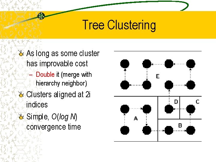
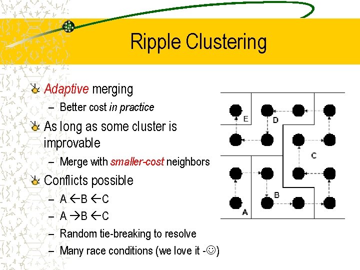
Tree Clustering As long as some cluster has improvable cost – Double it (merge with hierarchy neighbor) Clusters aligned at 2 i indices Simple, O(log N) convergence time

Ripple Clustering Adaptive merging – Better cost in practice As long as some cluster is improvable – Merge with smaller-cost neighbors Conflicts possible – – A B C Random tie-breaking to resolve Many race conditions (we love it - )

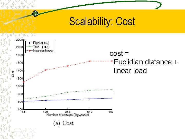
Scalability: Cost cost = Euclidian distance + linear load

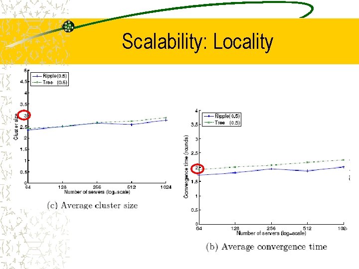
Scalability: Locality