
CS 1302 Computer Networks Unit 1 Data Communications
- Slides: 149
CS 1302 Computer Networks — Unit - 1 — — Data Communications — n Text Book Behrouz. A. Forouzan, “Data communication and Networking”, Tata Mc. Graw. Hill, 2004 11/25/2020 Unit-1 : Data Communications 1
Overview of Data Communications and Networking 11/25/2020 Unit-1 : Data Communications 2
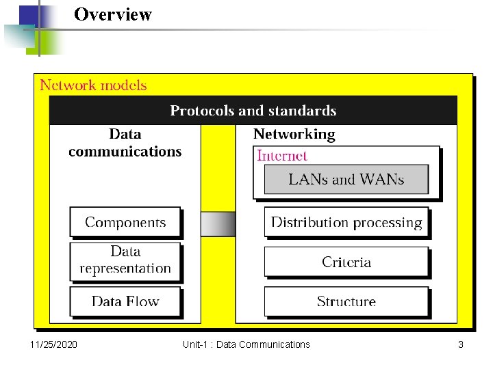
Overview 11/25/2020 Unit-1 : Data Communications 3
Introduction 11/25/2020 Unit-1 : Data Communications 4
1. 1 Data Communication Components Data Representation Direction of Data Flow 11/25/2020 Unit-1 : Data Communications 5
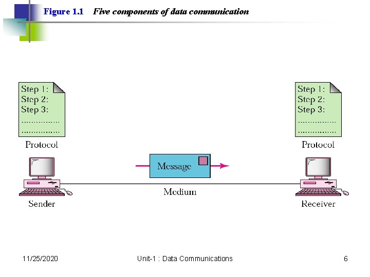
Figure 1. 1 11/25/2020 Five components of data communication Unit-1 : Data Communications 6
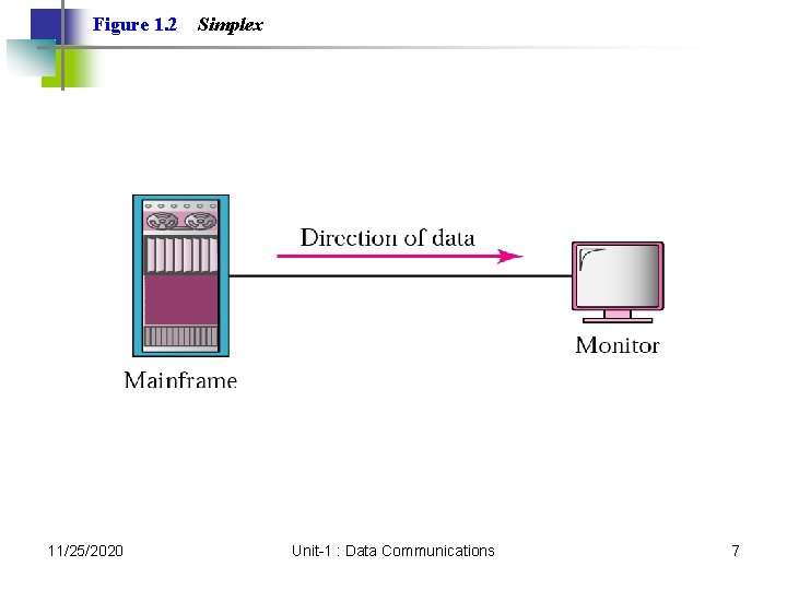
Figure 1. 2 11/25/2020 Simplex Unit-1 : Data Communications 7
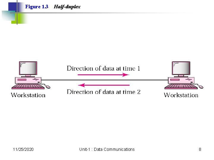
Figure 1. 3 11/25/2020 Half-duplex Unit-1 : Data Communications 8
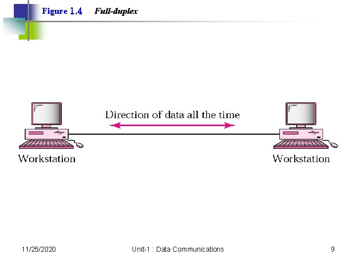
Figure 1. 4 11/25/2020 Full-duplex Unit-1 : Data Communications 9
1. 2 Networks Distributed Processing Network Criteria Physical Structures Categories of Networks 11/25/2020 Unit-1 : Data Communications 10
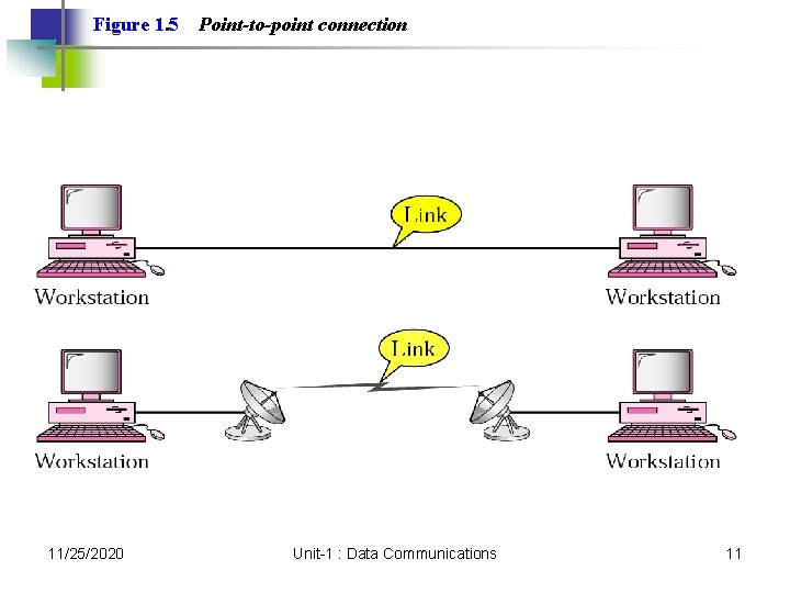
Figure 1. 5 11/25/2020 Point-to-point connection Unit-1 : Data Communications 11
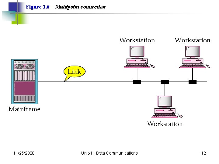
Figure 1. 6 11/25/2020 Multipoint connection Unit-1 : Data Communications 12
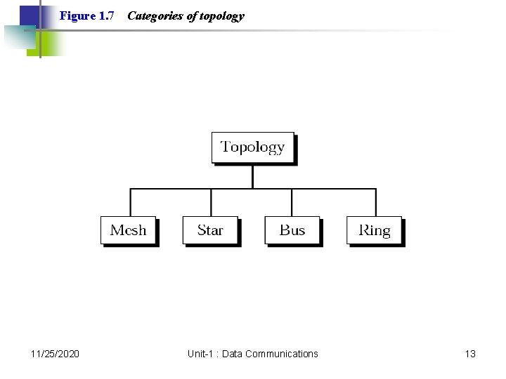
Figure 1. 7 11/25/2020 Categories of topology Unit-1 : Data Communications 13
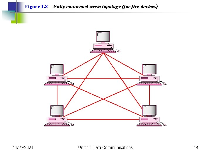
Figure 1. 8 11/25/2020 Fully connected mesh topology (for five devices) Unit-1 : Data Communications 14
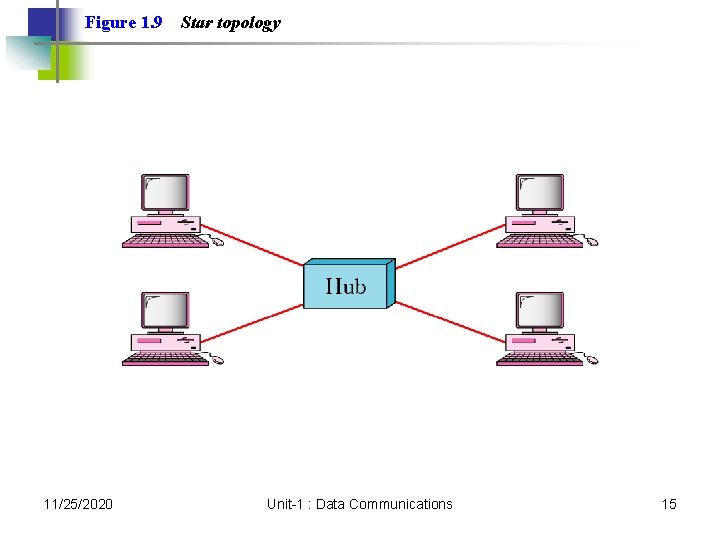
Figure 1. 9 11/25/2020 Star topology Unit-1 : Data Communications 15
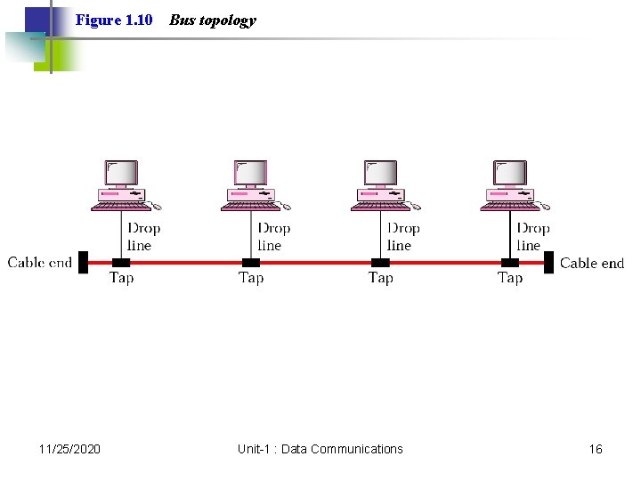
Figure 1. 10 11/25/2020 Bus topology Unit-1 : Data Communications 16
Figure 1. 11 11/25/2020 Ring topology Unit-1 : Data Communications 17
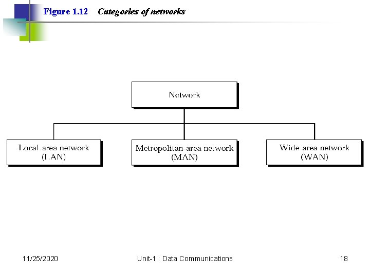
Figure 1. 12 11/25/2020 Categories of networks Unit-1 : Data Communications 18
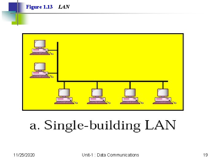
Figure 1. 13 11/25/2020 LAN Unit-1 : Data Communications 19
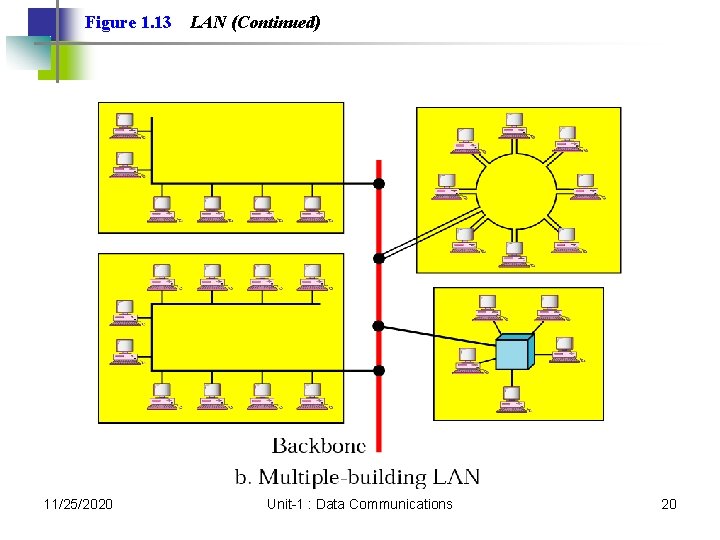
Figure 1. 13 11/25/2020 LAN (Continued) Unit-1 : Data Communications 20
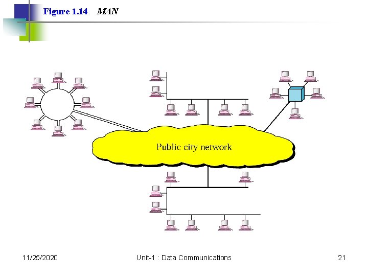
Figure 1. 14 11/25/2020 MAN Unit-1 : Data Communications 21
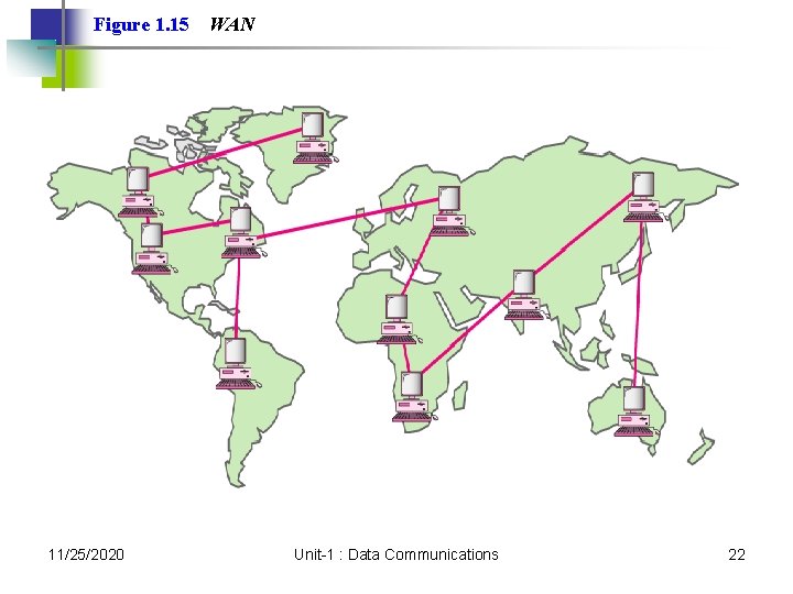
Figure 1. 15 11/25/2020 WAN Unit-1 : Data Communications 22
1. 3 The Internet A Brief History The Internet Today 11/25/2020 Unit-1 : Data Communications 23
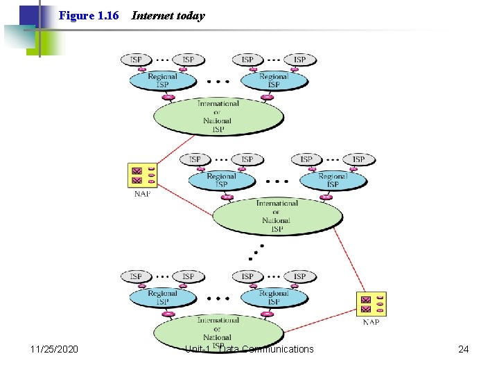
Figure 1. 16 11/25/2020 Internet today Unit-1 : Data Communications 24
1. 4 Protocols and Standards Protocols Standards Organizations Internet Standards 11/25/2020 Unit-1 : Data Communications 25
Network Models 11/25/2020 Unit-1 : Data Communications 26
2. 1 Layered Tasks Sender, Receiver, and Carrier Hierarchy Services 11/25/2020 Unit-1 : Data Communications 27
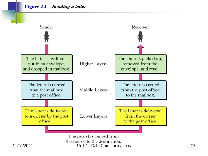
Figure 2. 1 11/25/2020 Sending a letter Unit-1 : Data Communications 28
2. 2 Internet Model Peer-to-Peer Processes Functions of Layers Summary of Layers 11/25/2020 Unit-1 : Data Communications 29
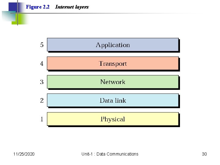
Figure 2. 2 11/25/2020 Internet layers Unit-1 : Data Communications 30
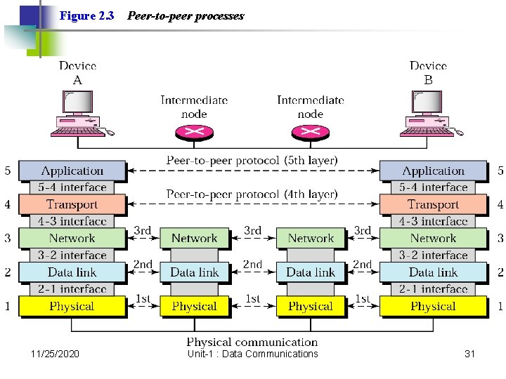
Figure 2. 3 11/25/2020 Peer-to-peer processes Unit-1 : Data Communications 31
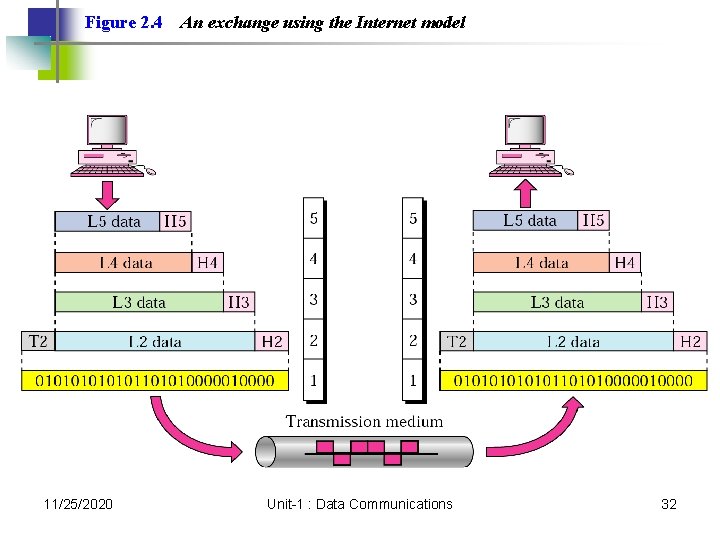
Figure 2. 4 11/25/2020 An exchange using the Internet model Unit-1 : Data Communications 32
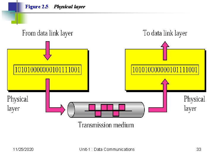
Figure 2. 5 11/25/2020 Physical layer Unit-1 : Data Communications 33
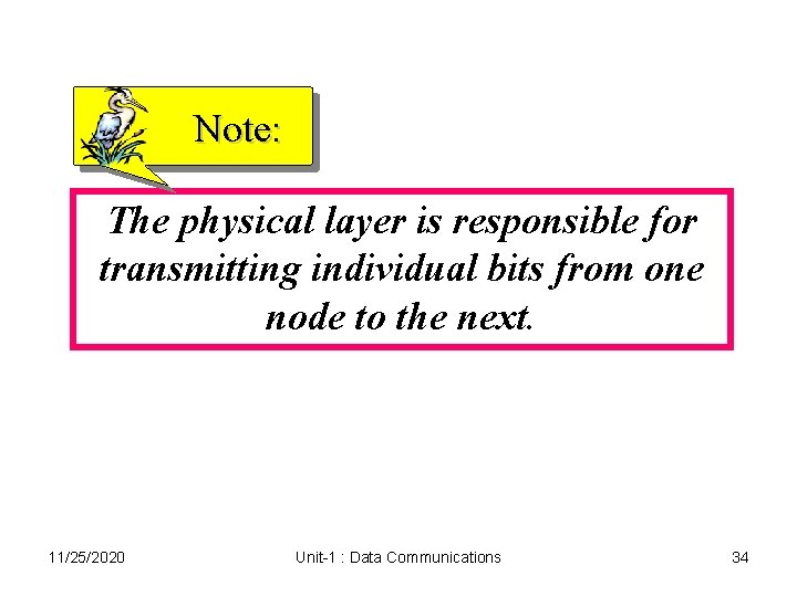
Note: The physical layer is responsible for transmitting individual bits from one node to the next. 11/25/2020 Unit-1 : Data Communications 34
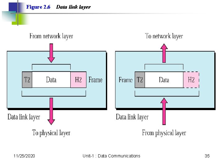
Figure 2. 6 11/25/2020 Data link layer Unit-1 : Data Communications 35
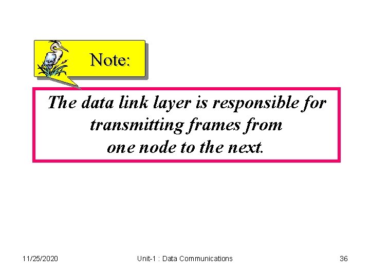
Note: The data link layer is responsible for transmitting frames from one node to the next. 11/25/2020 Unit-1 : Data Communications 36
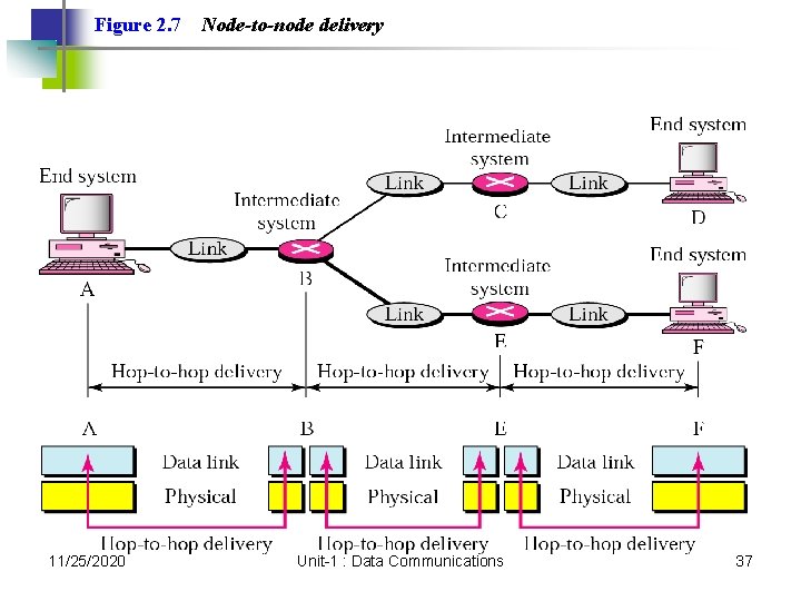
Figure 2. 7 11/25/2020 Node-to-node delivery Unit-1 : Data Communications 37
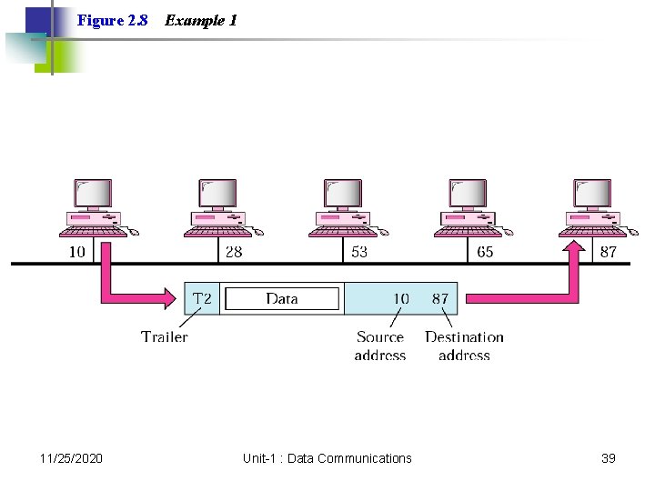
Example 1 In Figure 2. 8 a node with physical address 10 sends a frame to a node with physical address 87. The two nodes are connected by a link. At the data link level this frame contains physical addresses in the header. These are the only addresses needed. The rest of the header contains other information needed at this level. The trailer usually contains extra bits needed for error detection 11/25/2020 Unit-1 : Data Communications 38
Figure 2. 8 11/25/2020 Example 1 Unit-1 : Data Communications 39
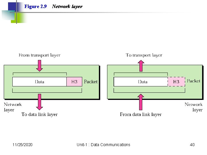
Figure 2. 9 11/25/2020 Network layer Unit-1 : Data Communications 40
Note: The network layer is responsible for the delivery of packets from the original source to the final destination. 11/25/2020 Unit-1 : Data Communications 41
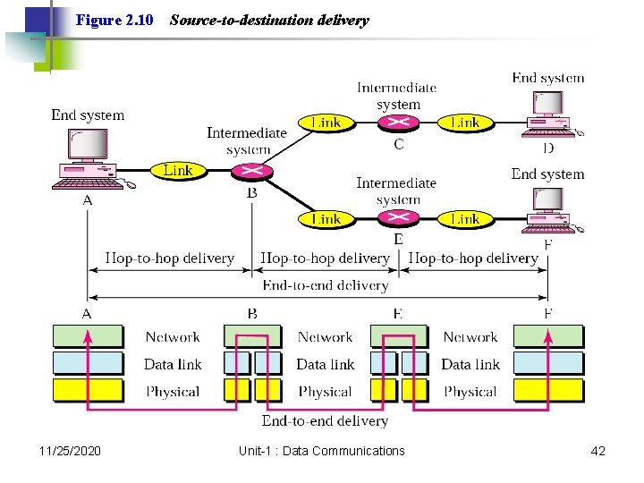
Figure 2. 10 11/25/2020 Source-to-destination delivery Unit-1 : Data Communications 42
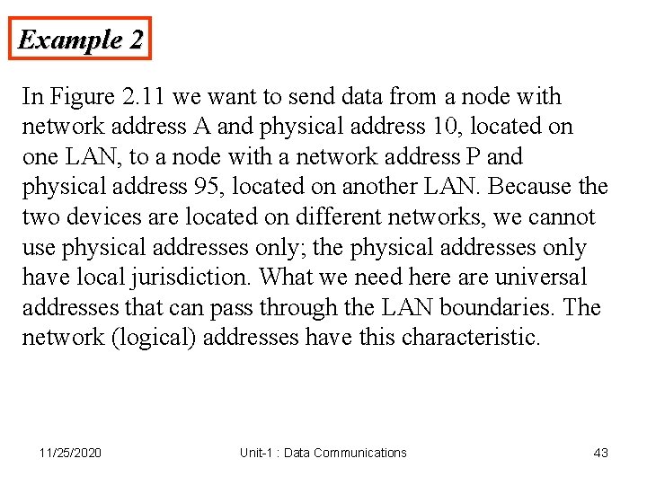
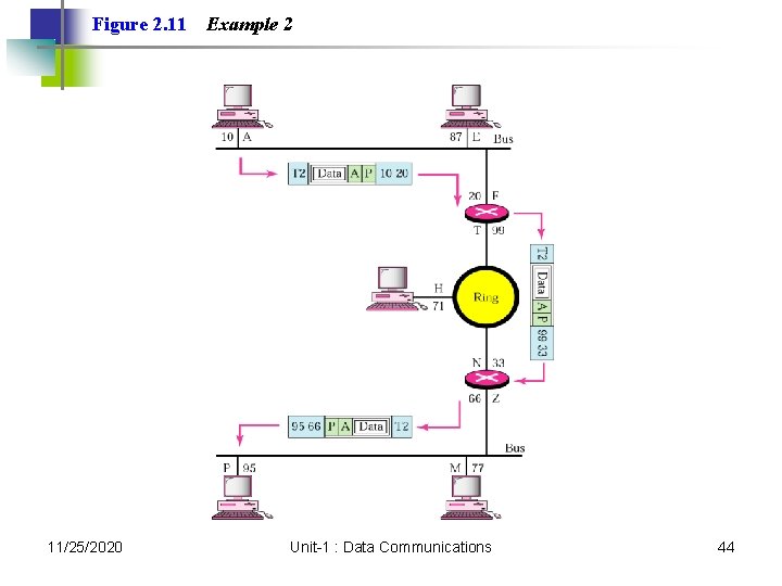
Example 2 In Figure 2. 11 we want to send data from a node with network address A and physical address 10, located on one LAN, to a node with a network address P and physical address 95, located on another LAN. Because the two devices are located on different networks, we cannot use physical addresses only; the physical addresses only have local jurisdiction. What we need here are universal addresses that can pass through the LAN boundaries. The network (logical) addresses have this characteristic. 11/25/2020 Unit-1 : Data Communications 43
Figure 2. 11 11/25/2020 Example 2 Unit-1 : Data Communications 44
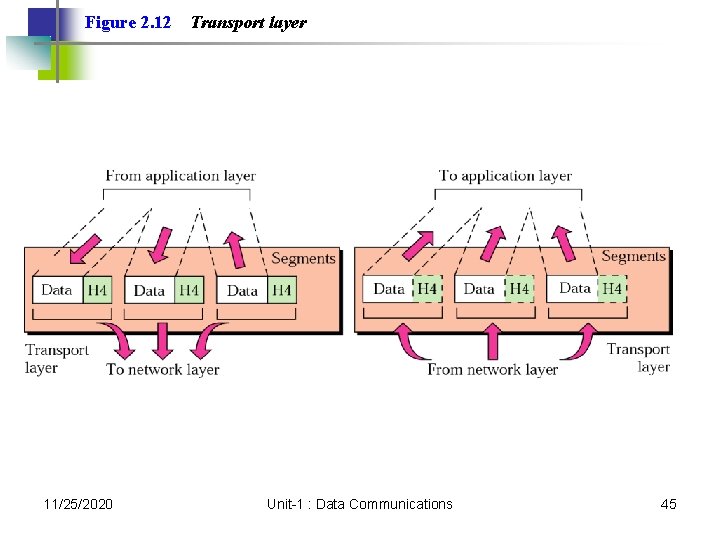
Figure 2. 12 11/25/2020 Transport layer Unit-1 : Data Communications 45
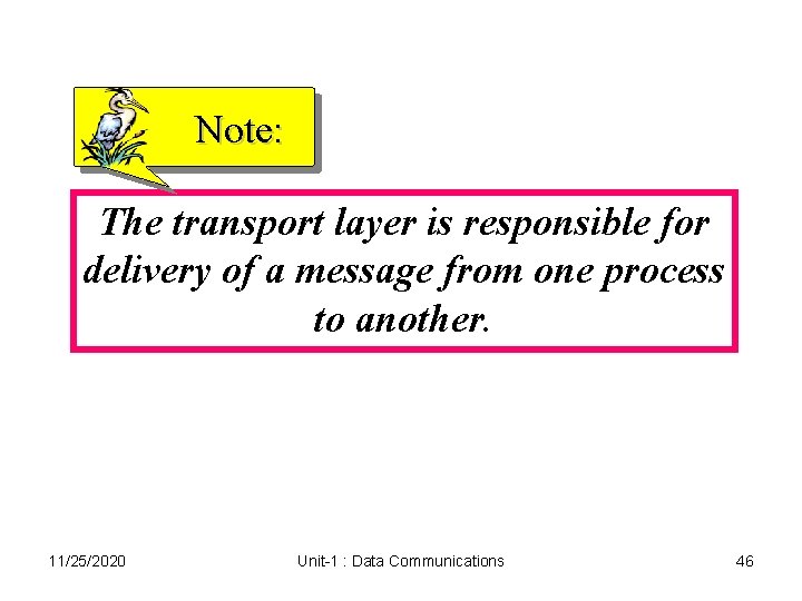
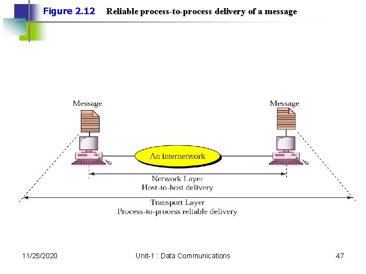
Note: The transport layer is responsible for delivery of a message from one process to another. 11/25/2020 Unit-1 : Data Communications 46
Figure 2. 12 11/25/2020 Reliable process-to-process delivery of a message Unit-1 : Data Communications 47
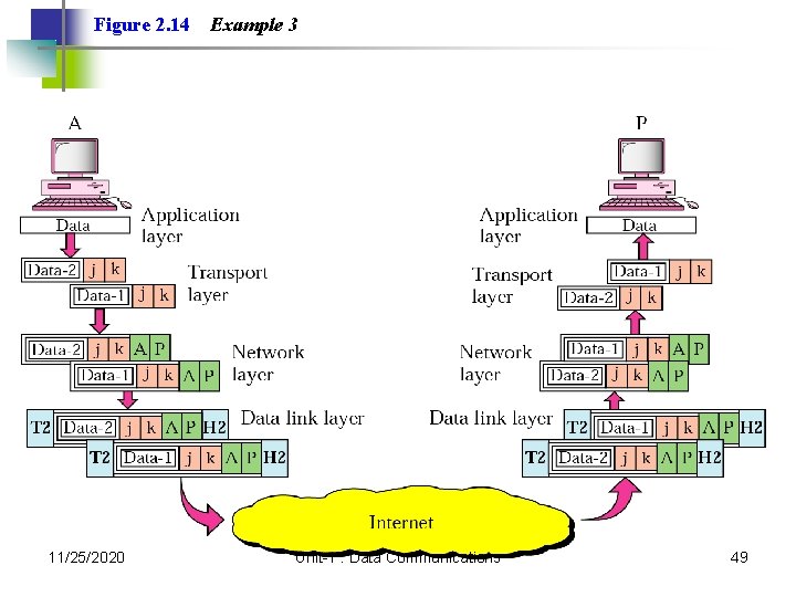
Example 3 Figure 2. 14 shows an example of transport layer communication. Data coming from the upper layers have port addresses j and k (j is the address of the sending process, and k is the address of the receiving process). Since the data size is larger than the network layer can handle, the data are split into two packets, each packet retaining the port addresses (j and k). Then in the network layer, network addresses (A and P) are added to each packet. 11/25/2020 Unit-1 : Data Communications 48
Figure 2. 14 11/25/2020 Example 3 Unit-1 : Data Communications 49
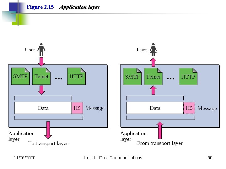
Figure 2. 15 11/25/2020 Application layer Unit-1 : Data Communications 50
Note: The application layer is responsible for providing services to the user. 11/25/2020 Unit-1 : Data Communications 51
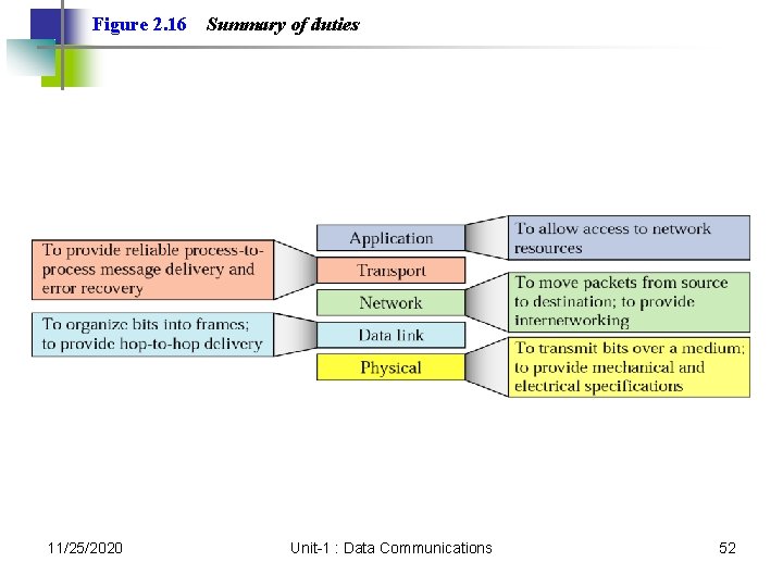
Figure 2. 16 11/25/2020 Summary of duties Unit-1 : Data Communications 52
2. 3 OSI Model A comparison 11/25/2020 Unit-1 : Data Communications 53
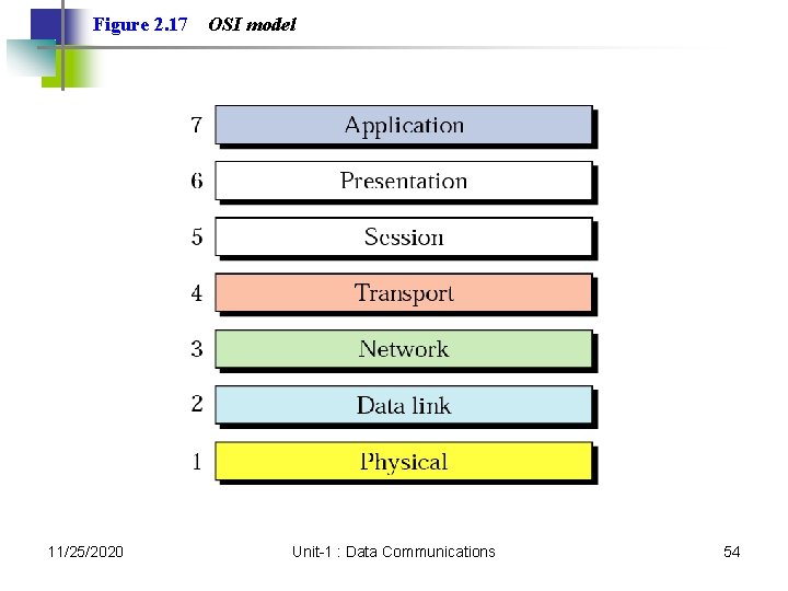
Figure 2. 17 11/25/2020 OSI model Unit-1 : Data Communications 54
Digital Transmission 11/25/2020 Unit-1 : Data Communications 55
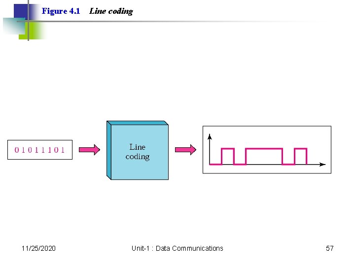
4. 1 Line Coding Some Characteristics Line Coding Schemes Some Other Schemes 11/25/2020 Unit-1 : Data Communications 56
Figure 4. 1 11/25/2020 Line coding Unit-1 : Data Communications 57
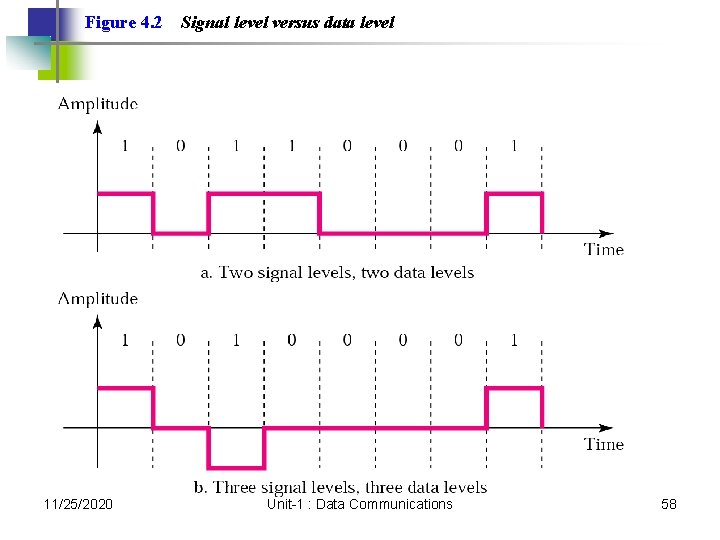
Figure 4. 2 11/25/2020 Signal level versus data level Unit-1 : Data Communications 58
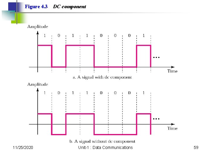
Figure 4. 3 11/25/2020 DC component Unit-1 : Data Communications 59
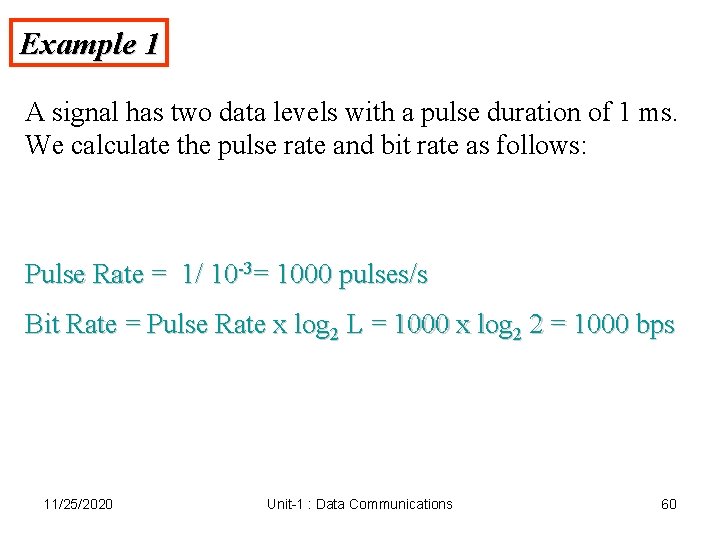
Example 1 A signal has two data levels with a pulse duration of 1 ms. We calculate the pulse rate and bit rate as follows: Pulse Rate = 1/ 10 -3= 1000 pulses/s Bit Rate = Pulse Rate x log 2 L = 1000 x log 2 2 = 1000 bps 11/25/2020 Unit-1 : Data Communications 60
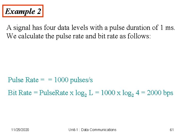
Example 2 A signal has four data levels with a pulse duration of 1 ms. We calculate the pulse rate and bit rate as follows: Pulse Rate = = 1000 pulses/s Bit Rate = Pulse. Rate x log 2 L = 1000 x log 2 4 = 2000 bps 11/25/2020 Unit-1 : Data Communications 61
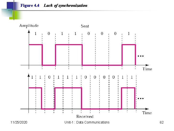
Figure 4. 4 11/25/2020 Lack of synchronization Unit-1 : Data Communications 62
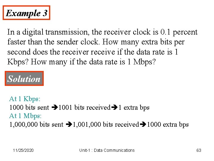
Example 3 In a digital transmission, the receiver clock is 0. 1 percent faster than the sender clock. How many extra bits per second does the receiver receive if the data rate is 1 Kbps? How many if the data rate is 1 Mbps? Solution At 1 Kbps: 1000 bits sent 1001 bits received 1 extra bps At 1 Mbps: 1, 000 bits sent 1, 000 bits received 1000 extra bps 11/25/2020 Unit-1 : Data Communications 63
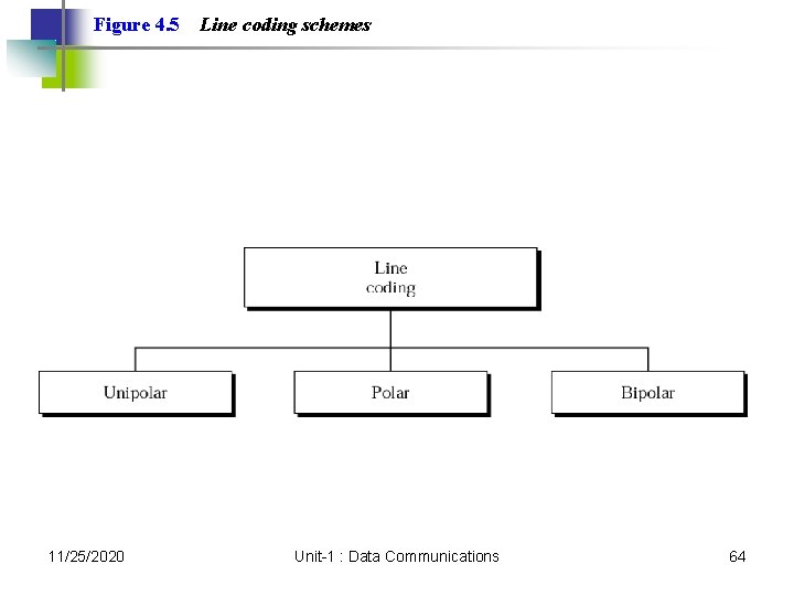
Figure 4. 5 11/25/2020 Line coding schemes Unit-1 : Data Communications 64
Note: Unipolar encoding uses only one voltage level. 11/25/2020 Unit-1 : Data Communications 65
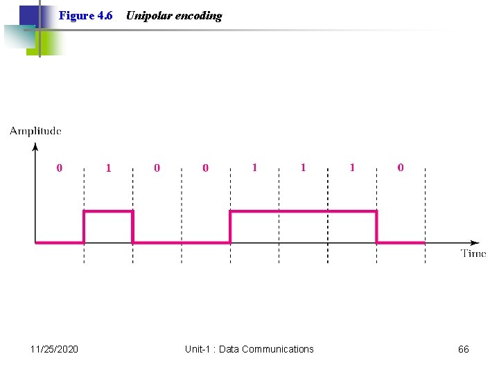
Figure 4. 6 11/25/2020 Unipolar encoding Unit-1 : Data Communications 66
Note: Polar encoding uses two voltage levels (positive and negative). 11/25/2020 Unit-1 : Data Communications 67
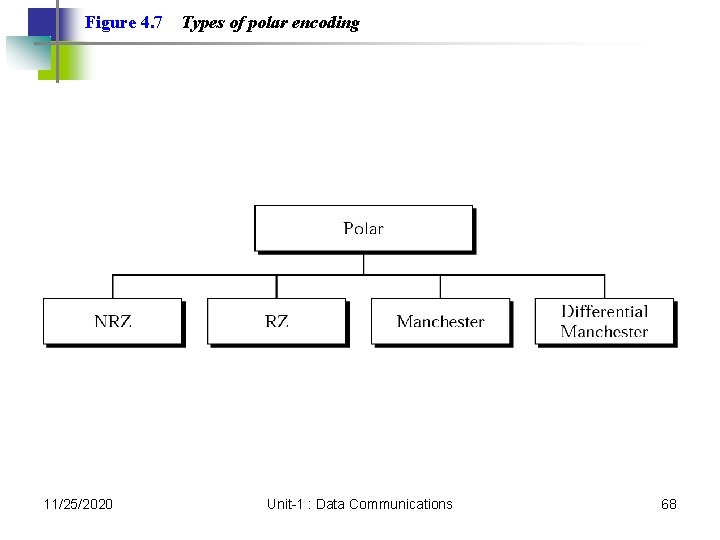
Figure 4. 7 11/25/2020 Types of polar encoding Unit-1 : Data Communications 68
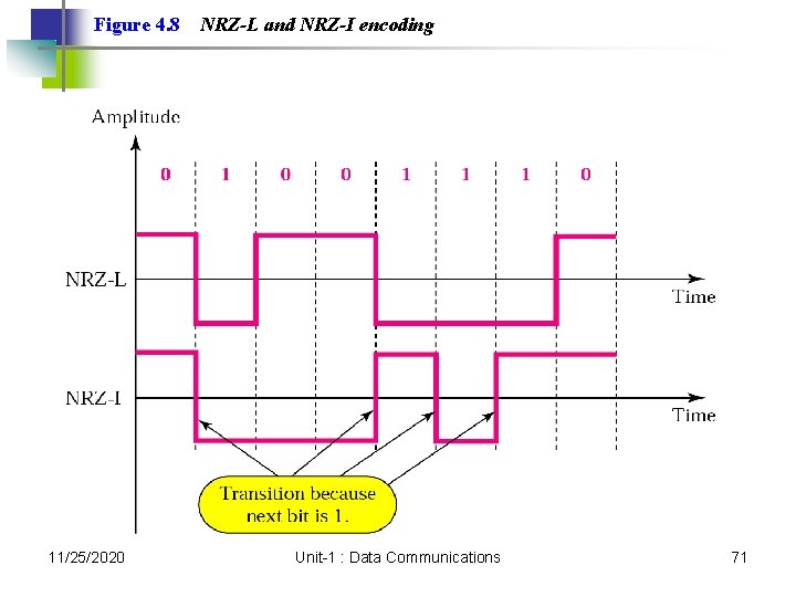
Note: In NRZ-L the level of the signal is dependent upon the state of the bit. 11/25/2020 Unit-1 : Data Communications 69
Note: In NRZ-I the signal is inverted if a 1 is encountered. 11/25/2020 Unit-1 : Data Communications 70
Figure 4. 8 11/25/2020 NRZ-L and NRZ-I encoding Unit-1 : Data Communications 71
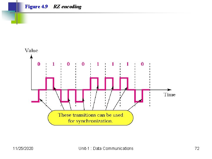
Figure 4. 9 11/25/2020 RZ encoding Unit-1 : Data Communications 72
Note: A good encoded digital signal must contain a provision for synchronization. 11/25/2020 Unit-1 : Data Communications 73
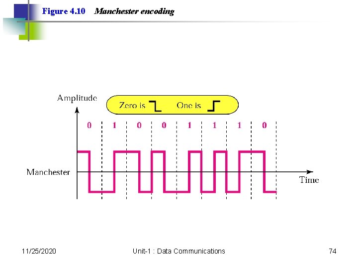
Figure 4. 10 11/25/2020 Manchester encoding Unit-1 : Data Communications 74
Note: In Manchester encoding, the transition at the middle of the bit is used for both synchronization and bit representation. 11/25/2020 Unit-1 : Data Communications 75
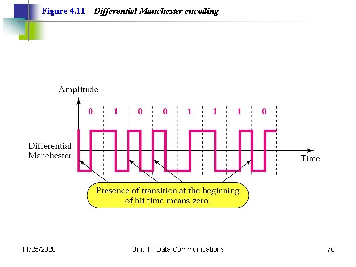
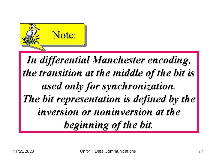
Figure 4. 11 11/25/2020 Differential Manchester encoding Unit-1 : Data Communications 76
Note: In differential Manchester encoding, the transition at the middle of the bit is used only for synchronization. The bit representation is defined by the inversion or noninversion at the beginning of the bit. 11/25/2020 Unit-1 : Data Communications 77
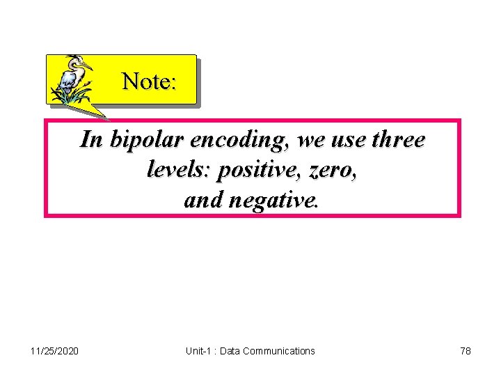
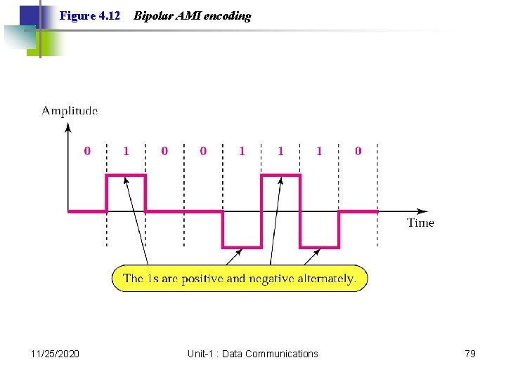
Note: In bipolar encoding, we use three levels: positive, zero, and negative. 11/25/2020 Unit-1 : Data Communications 78
Figure 4. 12 11/25/2020 Bipolar AMI encoding Unit-1 : Data Communications 79
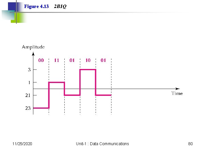
Figure 4. 13 11/25/2020 2 B 1 Q Unit-1 : Data Communications 80
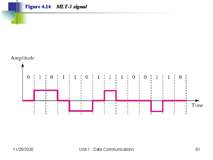
Figure 4. 14 11/25/2020 MLT-3 signal Unit-1 : Data Communications 81
4. 2 Block Coding Steps in Transformation Some Common Block Codes 11/25/2020 Unit-1 : Data Communications 82
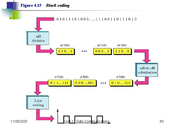
Figure 4. 15 11/25/2020 Block coding Unit-1 : Data Communications 83
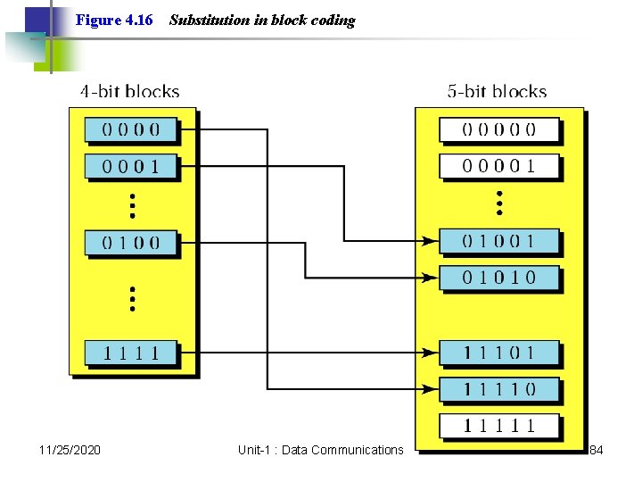
Figure 4. 16 11/25/2020 Substitution in block coding Unit-1 : Data Communications 84
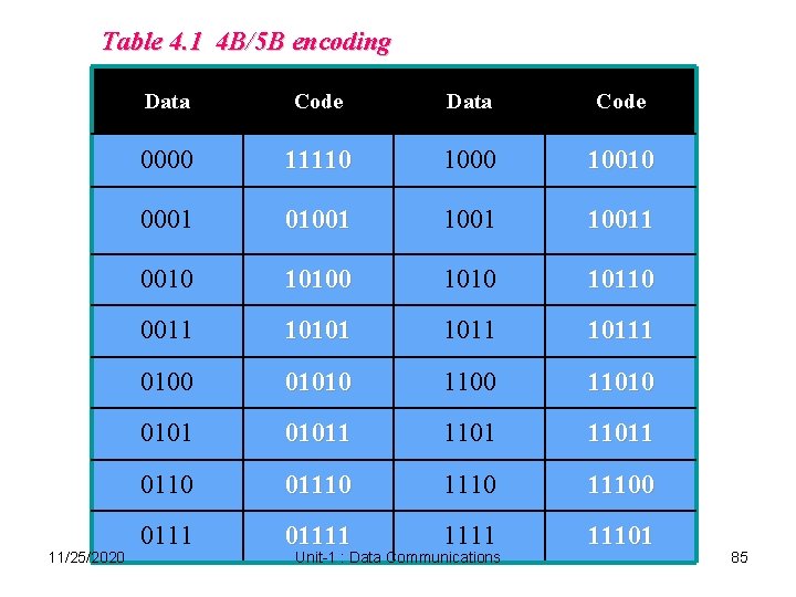
Table 4. 1 4 B/5 B encoding 11/25/2020 Data Code 0000 11110 10010 0001 010011 0010 1010 10110 0011 10101 10111 0100 01010 11010 01011 11011 0110 011100 01111 11101 Unit-1 : Data Communications 85
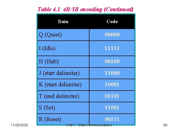
Table 4. 1 4 B/5 B encoding (Continued) Data 11/25/2020 Code Q (Quiet) 00000 I (Idle) 11111 H (Halt) 00100 J (start delimiter) 11000 K (start delimiter) 10001 T (end delimiter) 01101 S (Set) 11001 R (Reset) 00111 Unit-1 : Data Communications 86
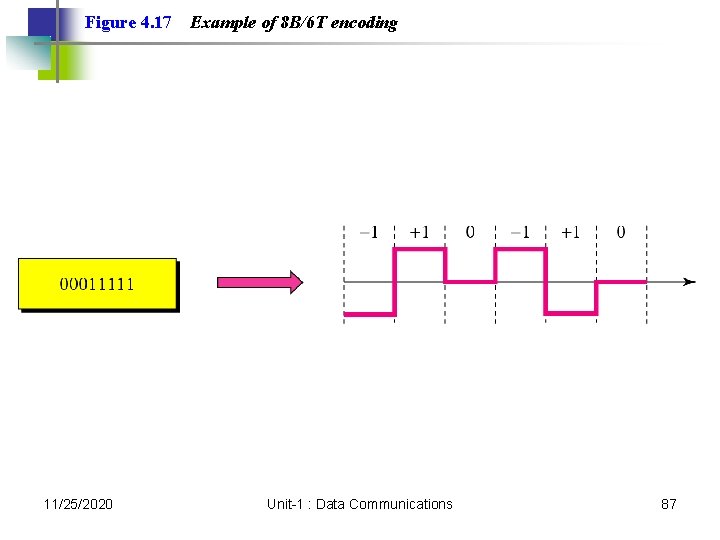
Figure 4. 17 11/25/2020 Example of 8 B/6 T encoding Unit-1 : Data Communications 87
4. 3 Sampling Pulse Amplitude Modulation Pulse Code Modulation Sampling Rate: Nyquist Theorem How Many Bits per Sample? Bit Rate 11/25/2020 Unit-1 : Data Communications 88
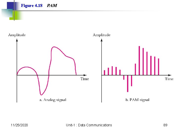
Figure 4. 18 11/25/2020 PAM Unit-1 : Data Communications 89
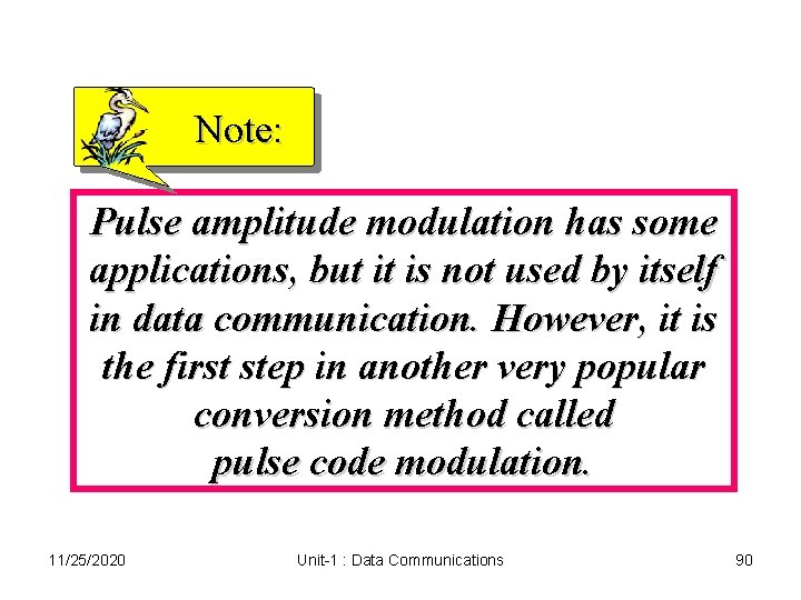
Note: Pulse amplitude modulation has some applications, but it is not used by itself in data communication. However, it is the first step in another very popular conversion method called pulse code modulation. 11/25/2020 Unit-1 : Data Communications 90
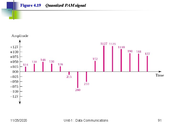
Figure 4. 19 11/25/2020 Quantized PAM signal Unit-1 : Data Communications 91
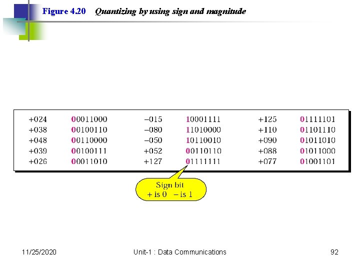
Figure 4. 20 11/25/2020 Quantizing by using sign and magnitude Unit-1 : Data Communications 92
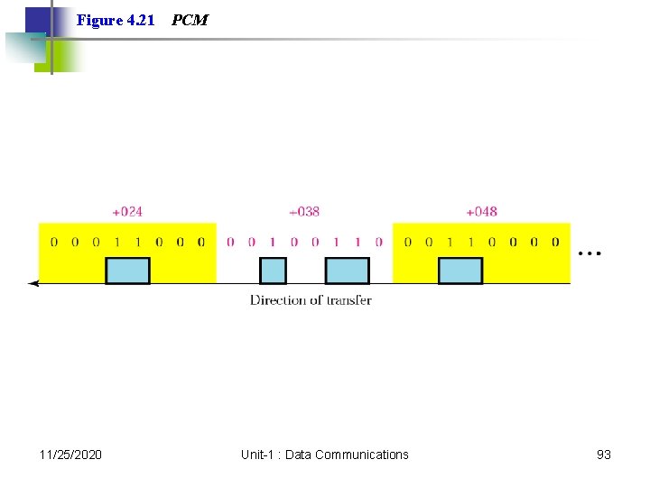
Figure 4. 21 11/25/2020 PCM Unit-1 : Data Communications 93
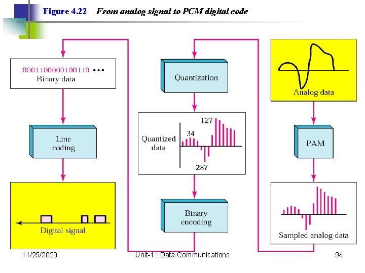
Figure 4. 22 11/25/2020 From analog signal to PCM digital code Unit-1 : Data Communications 94
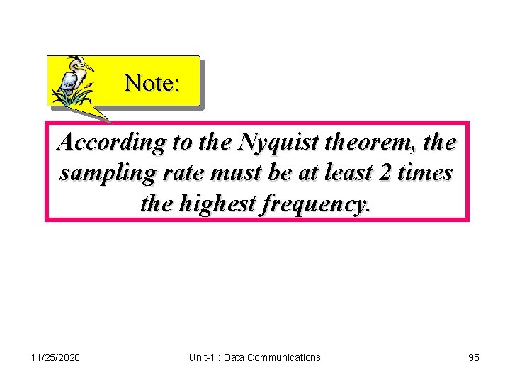
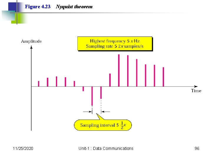
Note: According to the Nyquist theorem, the sampling rate must be at least 2 times the highest frequency. 11/25/2020 Unit-1 : Data Communications 95
Figure 4. 23 11/25/2020 Nyquist theorem Unit-1 : Data Communications 96
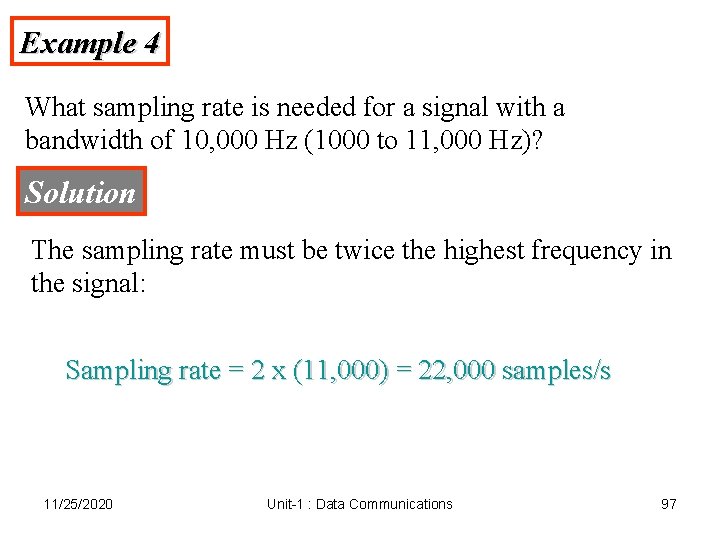
Example 4 What sampling rate is needed for a signal with a bandwidth of 10, 000 Hz (1000 to 11, 000 Hz)? Solution The sampling rate must be twice the highest frequency in the signal: Sampling rate = 2 x (11, 000) = 22, 000 samples/s 11/25/2020 Unit-1 : Data Communications 97
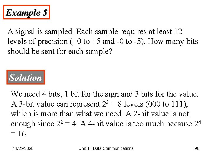
Example 5 A signal is sampled. Each sample requires at least 12 levels of precision (+0 to +5 and -0 to -5). How many bits should be sent for each sample? Solution We need 4 bits; 1 bit for the sign and 3 bits for the value. A 3 -bit value can represent 23 = 8 levels (000 to 111), which is more than what we need. A 2 -bit value is not enough since 22 = 4. A 4 -bit value is too much because 24 = 16. 11/25/2020 Unit-1 : Data Communications 98
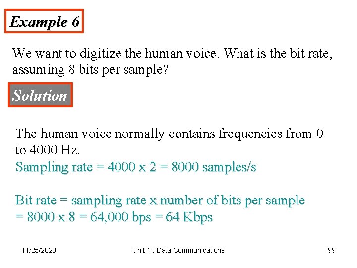
Example 6 We want to digitize the human voice. What is the bit rate, assuming 8 bits per sample? Solution The human voice normally contains frequencies from 0 to 4000 Hz. Sampling rate = 4000 x 2 = 8000 samples/s Bit rate = sampling rate x number of bits per sample = 8000 x 8 = 64, 000 bps = 64 Kbps 11/25/2020 Unit-1 : Data Communications 99
Note: Note that we can always change a band-pass signal to a low-pass signal before sampling. In this case, the sampling rate is twice the bandwidth. 11/25/2020 Unit-1 : Data Communications 100
4. 4 Transmission Mode Parallel Transmission Serial Transmission 11/25/2020 Unit-1 : Data Communications 101
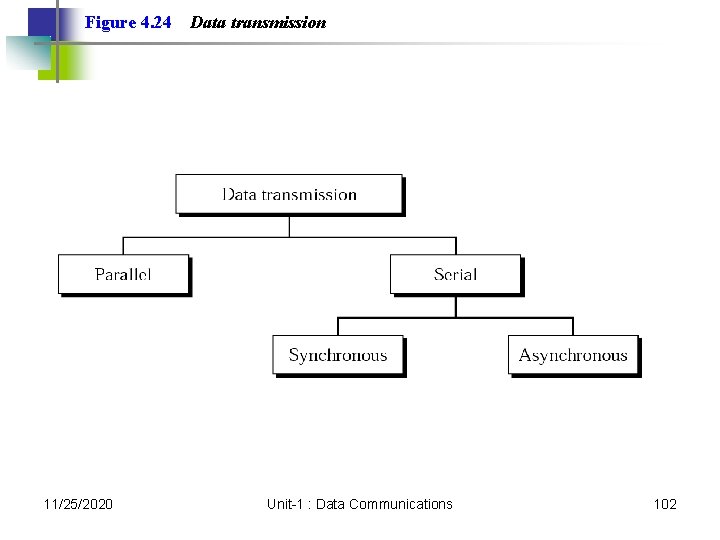
Figure 4. 24 11/25/2020 Data transmission Unit-1 : Data Communications 102
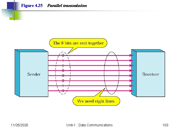
Figure 4. 25 11/25/2020 Parallel transmission Unit-1 : Data Communications 103
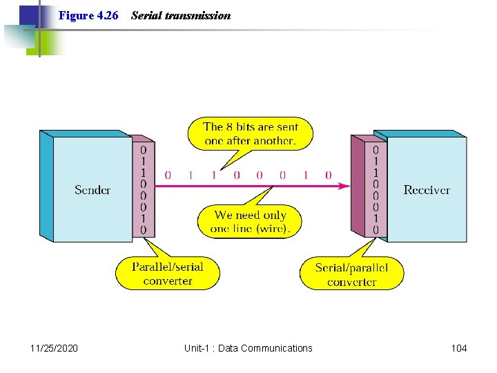
Figure 4. 26 11/25/2020 Serial transmission Unit-1 : Data Communications 104
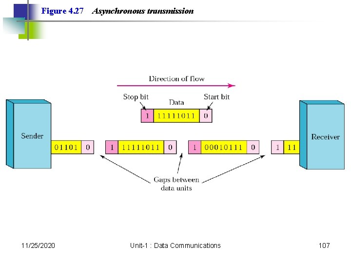
Note: In asynchronous transmission, we send 1 start bit (0) at the beginning and 1 or more stop bits (1 s) at the end of each byte. There may be a gap between each byte. 11/25/2020 Unit-1 : Data Communications 105
Note: Asynchronous here means “asynchronous at the byte level, ” but the bits are still synchronized; their durations are the same. 11/25/2020 Unit-1 : Data Communications 106
Figure 4. 27 11/25/2020 Asynchronous transmission Unit-1 : Data Communications 107
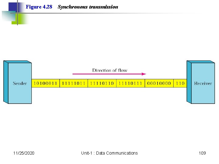
Note: In synchronous transmission, we send bits one after another without start/stop bits or gaps. It is the responsibility of the receiver to group the bits. 11/25/2020 Unit-1 : Data Communications 108
Figure 4. 28 11/25/2020 Synchronous transmission Unit-1 : Data Communications 109
5. 2 Telephone Modems Modem Standards 11/25/2020 Unit-1 : Data Communications 110
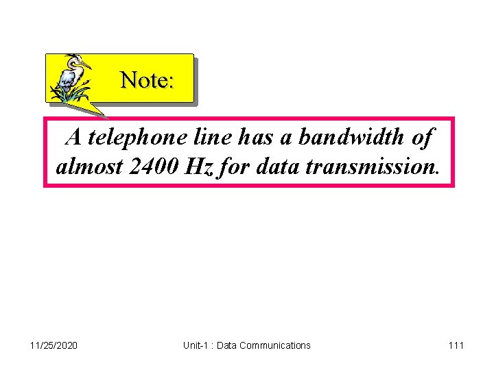
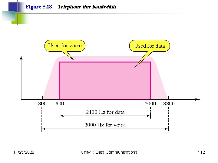
Note: A telephone line has a bandwidth of almost 2400 Hz for data transmission. 11/25/2020 Unit-1 : Data Communications 111
Figure 5. 18 11/25/2020 Telephone line bandwidth Unit-1 : Data Communications 112
Note: Modem stands for modulator/demodulator. 11/25/2020 Unit-1 : Data Communications 113
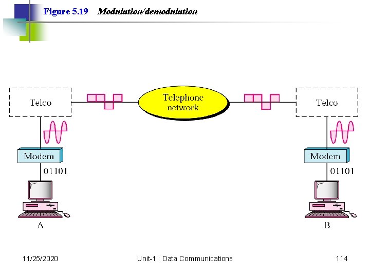
Figure 5. 19 11/25/2020 Modulation/demodulation Unit-1 : Data Communications 114
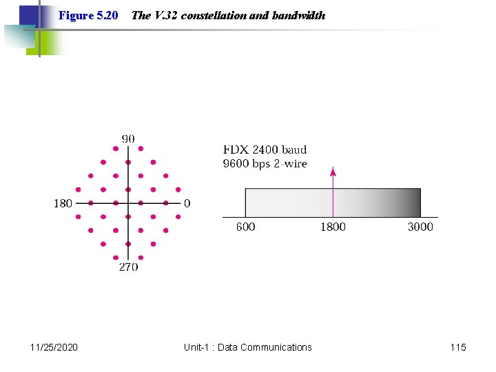
Figure 5. 20 11/25/2020 The V. 32 constellation and bandwidth Unit-1 : Data Communications 115
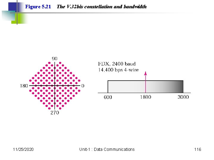
Figure 5. 21 11/25/2020 The V. 32 bis constellation and bandwidth Unit-1 : Data Communications 116
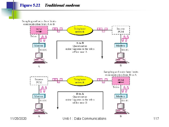
Figure 5. 22 11/25/2020 Traditional modems Unit-1 : Data Communications 117
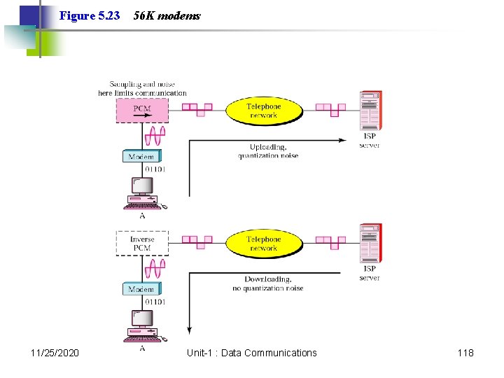
Figure 5. 23 11/25/2020 56 K modems Unit-1 : Data Communications 118
Transmission Media 11/25/2020 Unit-1 : Data Communications 119
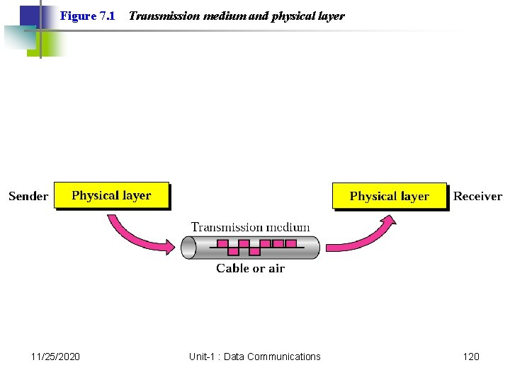
Figure 7. 1 11/25/2020 Transmission medium and physical layer Unit-1 : Data Communications 120
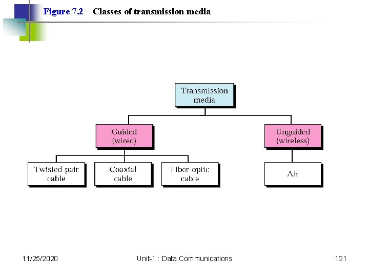
Figure 7. 2 11/25/2020 Classes of transmission media Unit-1 : Data Communications 121
7. 1 Guided Media Twisted-Pair Cable Coaxial Cable Fiber-Optic Cable 11/25/2020 Unit-1 : Data Communications 122
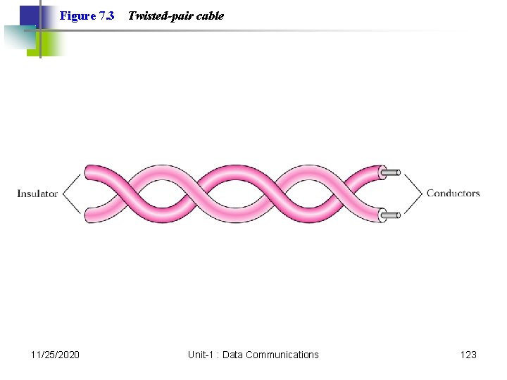
Figure 7. 3 11/25/2020 Twisted-pair cable Unit-1 : Data Communications 123
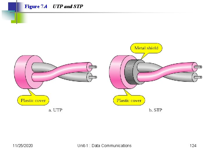
Figure 7. 4 11/25/2020 UTP and STP Unit-1 : Data Communications 124
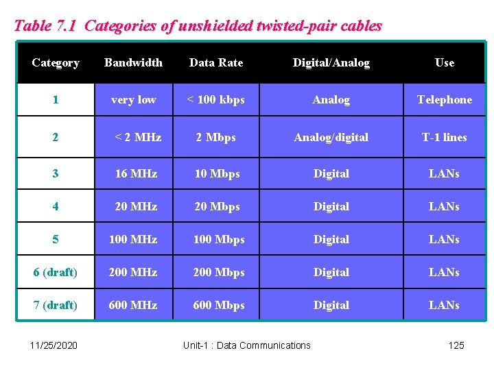
Table 7. 1 Categories of unshielded twisted-pair cables Category Bandwidth Data Rate Digital/Analog Use 1 very low < 100 kbps Analog Telephone 2 < 2 MHz 2 Mbps Analog/digital T-1 lines 3 16 MHz 10 Mbps Digital LANs 4 20 MHz 20 Mbps Digital LANs 5 100 MHz 100 Mbps Digital LANs 6 (draft) 200 MHz 200 Mbps Digital LANs 7 (draft) 600 MHz 600 Mbps Digital LANs 11/25/2020 Unit-1 : Data Communications 125
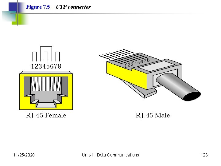
Figure 7. 5 11/25/2020 UTP connector Unit-1 : Data Communications 126
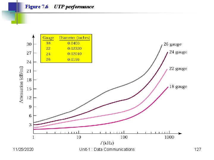
Figure 7. 6 11/25/2020 UTP performance Unit-1 : Data Communications 127
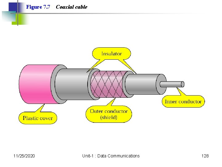
Figure 7. 7 11/25/2020 Coaxial cable Unit-1 : Data Communications 128
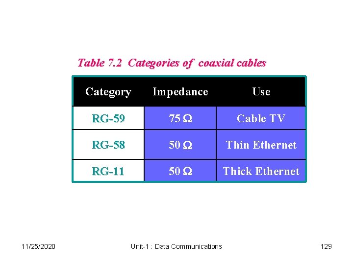
Table 7. 2 Categories of coaxial cables 11/25/2020 Category Impedance Use RG-59 75 W Cable TV RG-58 50 W Thin Ethernet RG-11 50 W Thick Ethernet Unit-1 : Data Communications 129
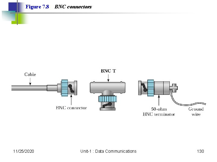
Figure 7. 8 11/25/2020 BNC connectors Unit-1 : Data Communications 130
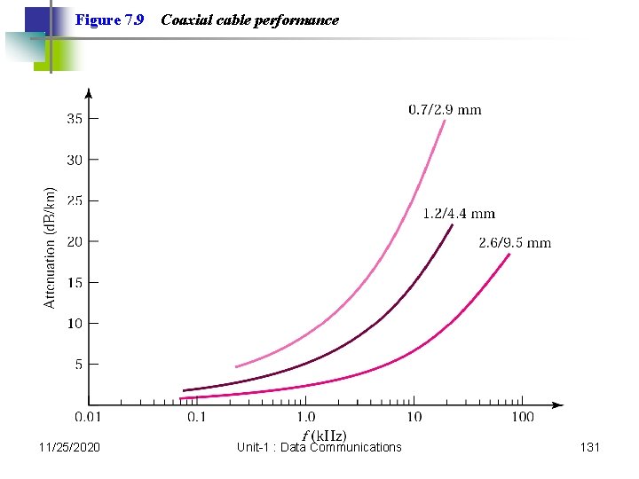
Figure 7. 9 11/25/2020 Coaxial cable performance Unit-1 : Data Communications 131
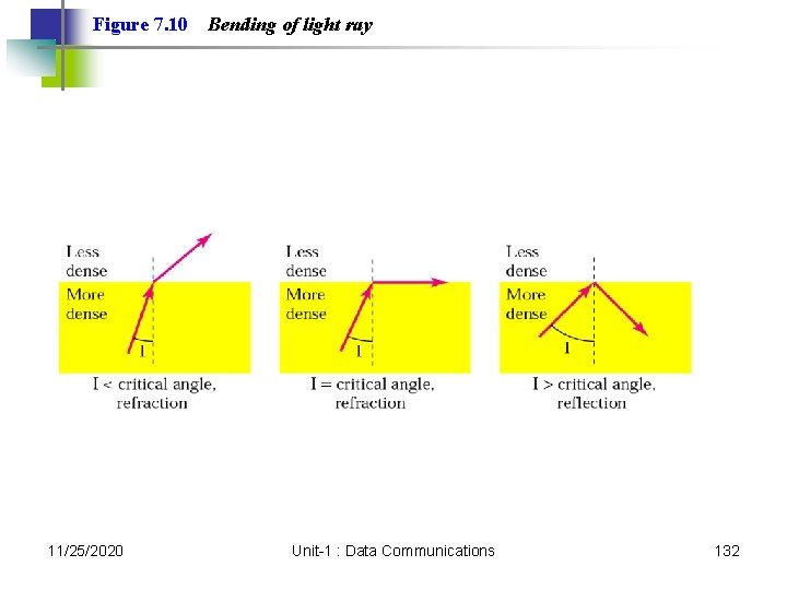
Figure 7. 10 11/25/2020 Bending of light ray Unit-1 : Data Communications 132
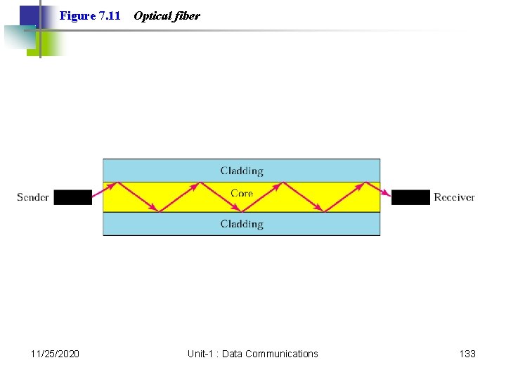
Figure 7. 11 11/25/2020 Optical fiber Unit-1 : Data Communications 133
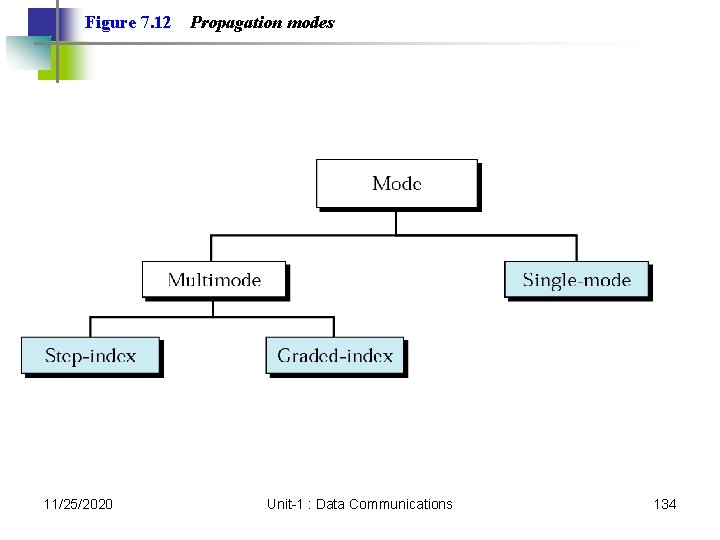
Figure 7. 12 11/25/2020 Propagation modes Unit-1 : Data Communications 134
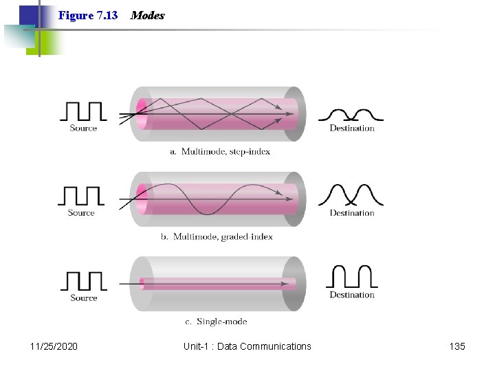
Figure 7. 13 11/25/2020 Modes Unit-1 : Data Communications 135
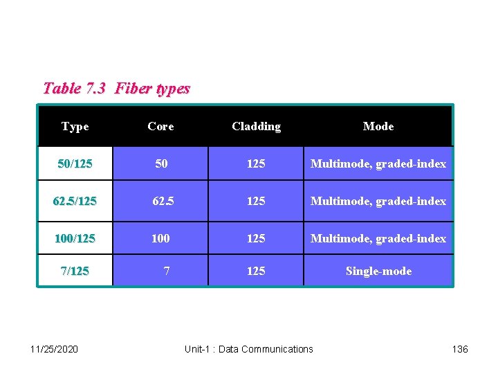
Table 7. 3 Fiber types Type Core Cladding Mode 50/125 50 125 Multimode, graded-index 62. 5/125 62. 5 125 Multimode, graded-index 100/125 100 125 Multimode, graded-index 7 125 Single-mode 7/125 11/25/2020 Unit-1 : Data Communications 136
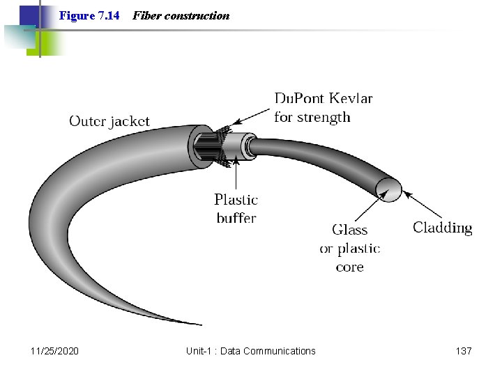
Figure 7. 14 11/25/2020 Fiber construction Unit-1 : Data Communications 137
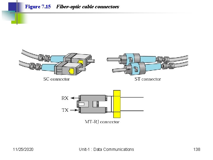
Figure 7. 15 11/25/2020 Fiber-optic cable connectors Unit-1 : Data Communications 138
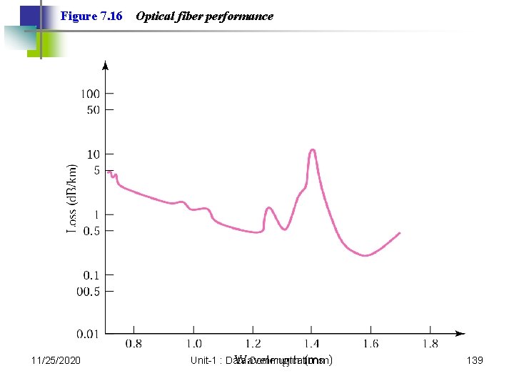
Figure 7. 16 11/25/2020 Optical fiber performance Unit-1 : Data Communications 139
7. 2 Unguided Media: Wireless Radio Waves Microwaves Infrared 11/25/2020 Unit-1 : Data Communications 140
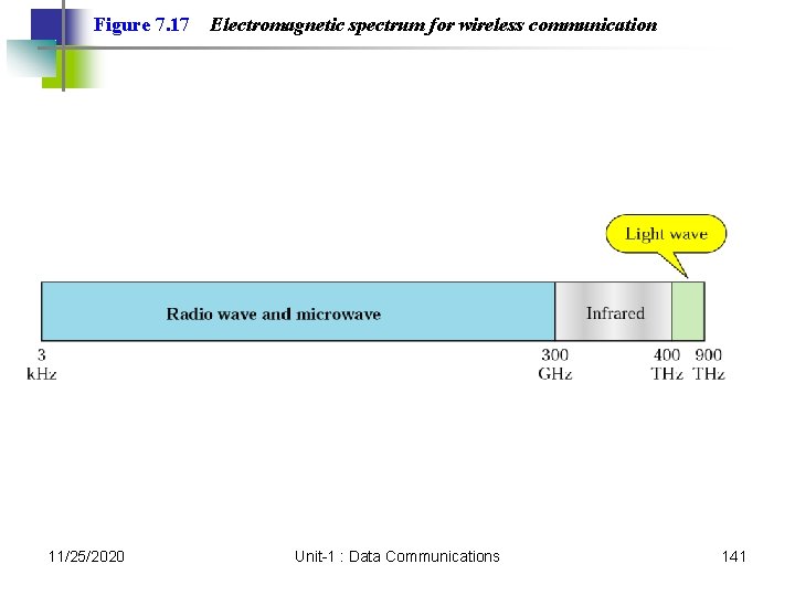
Figure 7. 17 11/25/2020 Electromagnetic spectrum for wireless communication Unit-1 : Data Communications 141
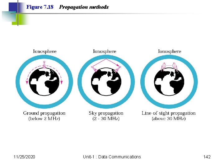
Figure 7. 18 11/25/2020 Propagation methods Unit-1 : Data Communications 142
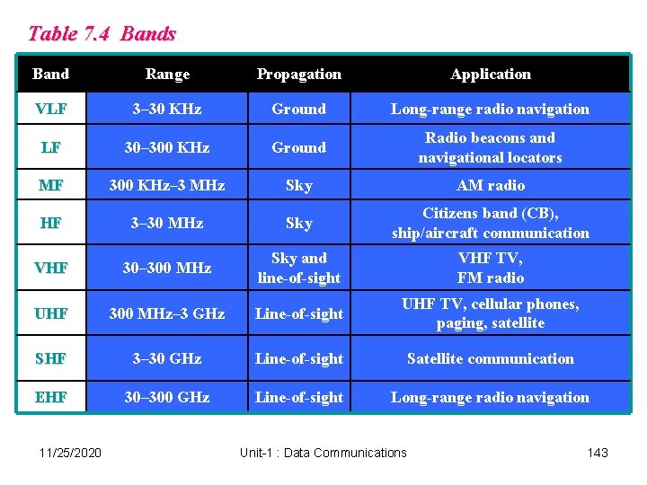
Table 7. 4 Bands Band Range Propagation Application VLF 3– 30 KHz Ground Long-range radio navigation LF 30– 300 KHz Ground Radio beacons and navigational locators MF 300 KHz– 3 MHz Sky AM radio HF 3– 30 MHz Sky Citizens band (CB), ship/aircraft communication VHF 30– 300 MHz Sky and line-of-sight VHF TV, FM radio UHF 300 MHz– 3 GHz Line-of-sight UHF TV, cellular phones, paging, satellite SHF 3– 30 GHz Line-of-sight Satellite communication EHF 30– 300 GHz Line-of-sight Long-range radio navigation 11/25/2020 Unit-1 : Data Communications 143
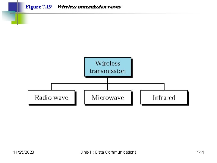
Figure 7. 19 11/25/2020 Wireless transmission waves Unit-1 : Data Communications 144
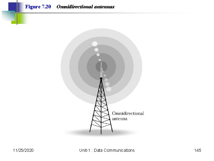
Figure 7. 20 11/25/2020 Omnidirectional antennas Unit-1 : Data Communications 145
Note: Radio waves are used for multicast communications, such as radio and television, and paging systems. 11/25/2020 Unit-1 : Data Communications 146
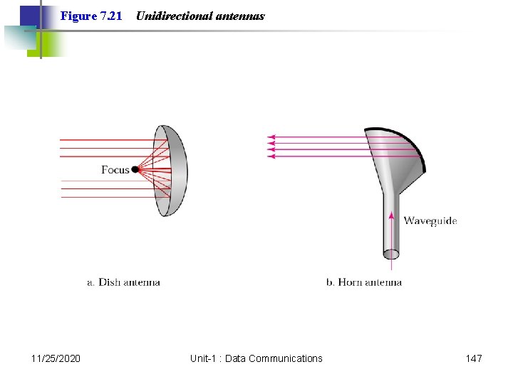
Figure 7. 21 11/25/2020 Unidirectional antennas Unit-1 : Data Communications 147
Note: Microwaves are used for unicast communication such as cellular telephones, satellite networks, and wireless LANs. 11/25/2020 Unit-1 : Data Communications 148
Note: Infrared signals can be used for shortrange communication in a closed area using line-of-sight propagation. 11/25/2020 Unit-1 : Data Communications 149