Technion Israel Institute of Technology Faculty of Aerospace

Technion – Israel Institute of Technology – Faculty of Aerospace Engineering Significance of Localized Vortical Disturbances in Wall-Bounded and Free Shear Flows Jacob Cohen 1, Ilia Shukhman 2 Michael Karp 1 and Jimmy Philip 1 1. Faculty of Aerospace Engineering, Technion, Haifa, Israel 2. Institute of Solar-Terrestrial Physics, Russian Academy of Sciences, Siberian Department, Irkutsk 664033, P. O. Box 4026, Russia

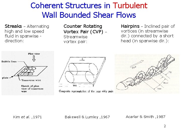
Coherent Structures in Turbulent Wall Bounded Shear Flows Streaks – Alternating high and low speed fluid in spanwise direction: Kim et al. , 1971 Counter Rotating Vortex Pair (CVP) – Streamwise vortex pair: Bakewell & Lumley , 1967 Hairpins – Inclined pair of vortices (in streamwise dir. ) connected by a short head (in spanwise dir. ): Acarlar & Smith , 1987 2

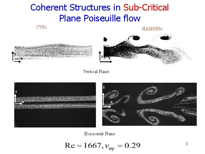
Coherent Structures in Sub-Critical Plane Poiseuille flow CVPs y x HAIRPINs y x Vertical Plane (b 1) z (b 2) x z x Horizontal Plane 3

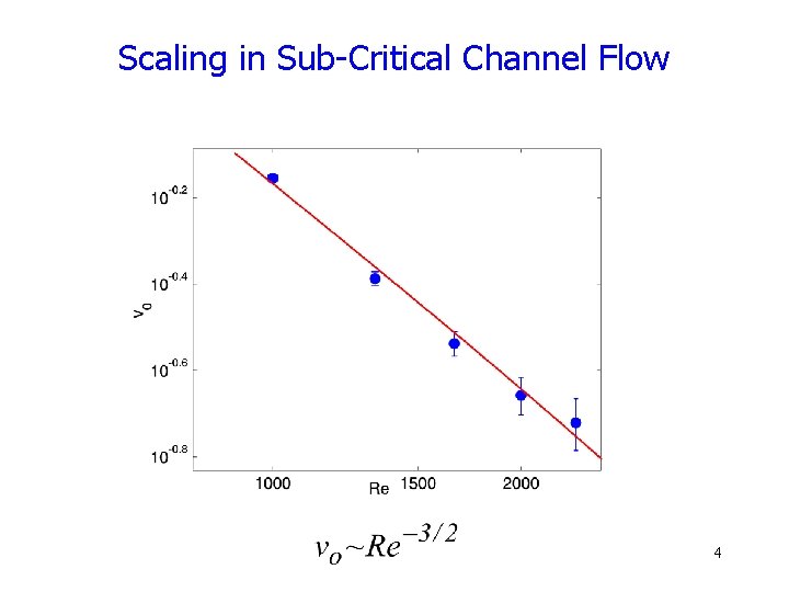
Scaling in Sub-Critical Channel Flow 4

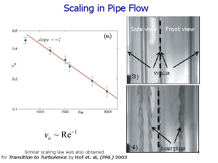
Scaling in Pipe Flow Side view Similar scaling law was also obtained for Transition to Turbulence by Hof et. al, (PRL) 2003 Front view 5

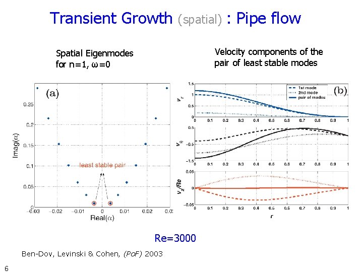
Transient Growth (spatial) Velocity components of the pair of least stable modes Spatial Eigenmodes for n=1, ω=0 Re=3000 Ben-Dov, Levinski & Cohen, (Po. F) 2003 6 : Pipe flow

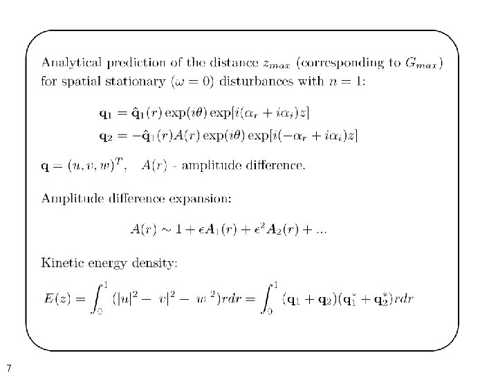
7

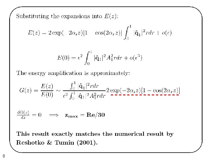
8

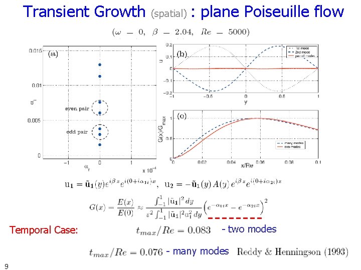
Transient Growth Temporal Case: (spatial) : plane Poiseuille flow - two modes - many modes 9

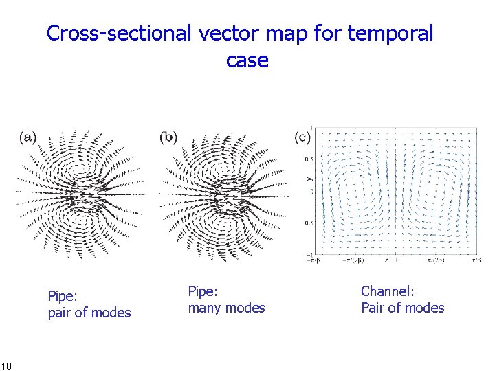
Cross-sectional vector map for temporal case Pipe: pair of modes 10 Pipe: many modes Channel: Pair of modes

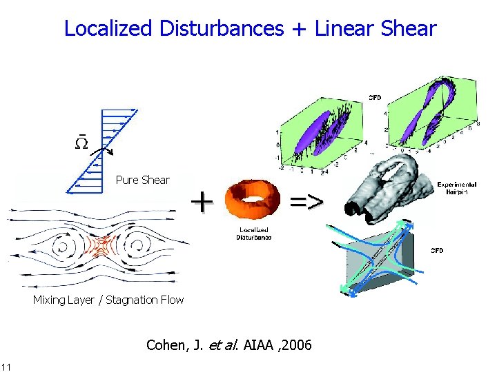
Localized Disturbances + Linear Shear Pure Shear Mixing Layer / Stagnation Flow Cohen, J. et al. AIAA , 2006 11

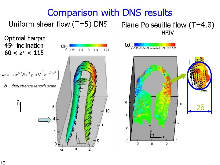
Comparison with DNS results Uniform shear flow (T=5) DNS Optimal hairpin 45 o inclination 60 < z+ < 115 Plane Poiseuille flow (T=4. 8) HPIV ωy - disturbance length scale 2δ 12

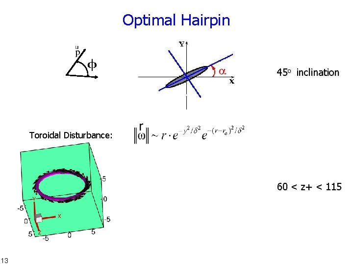
Optimal Hairpin 45 o inclination Toroidal Disturbance: 60 < z+ < 115 13

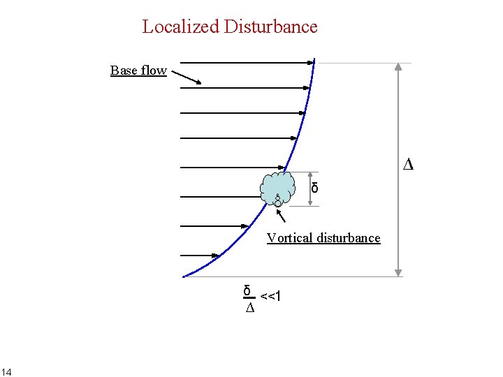
Localized Disturbance Base flow ∆ δ Vortical disturbance δ <<1 ∆ 14

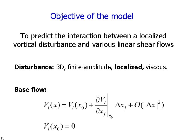
Objective of the model To predict the interaction between a localized vortical disturbance and various linear shear flows Disturbance: 3 D, finite-amplitude, localized, viscous. Base flow: 15

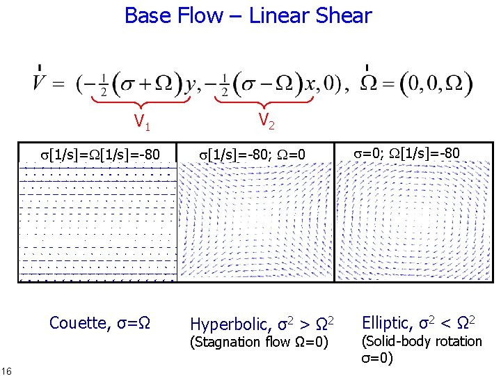
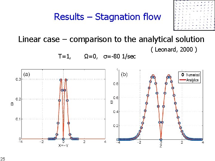
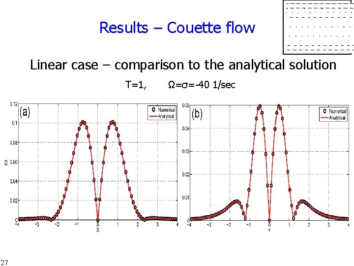
Base Flow – Linear Shear V 1 [1/s]=-80 Couette, σ=Ω V 2 [1/s]=-80; =0 Hyperbolic, σ2 > Ω 2 (Stagnation flow Ω=0) 16 =0; [1/s]=-80 Elliptic, σ2 < Ω 2 (Solid-body rotation σ=0)

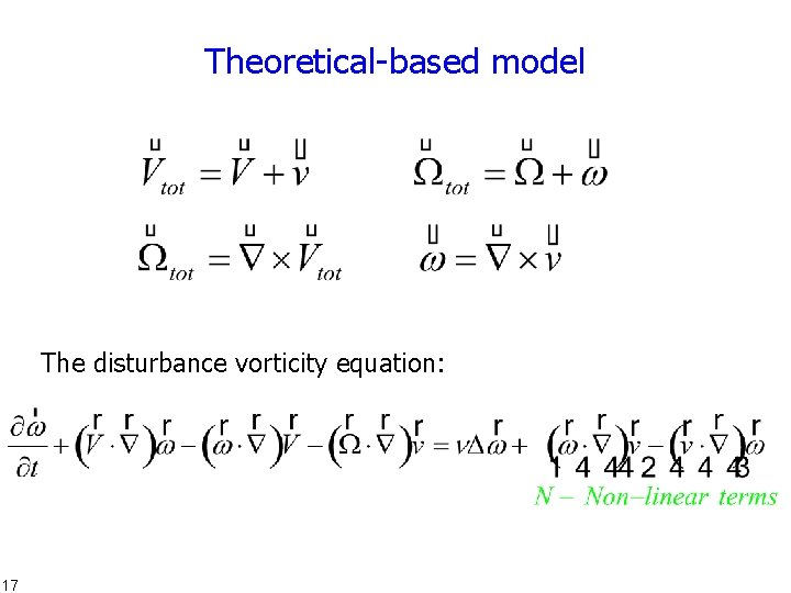
Theoretical-based model The disturbance vorticity equation: 17

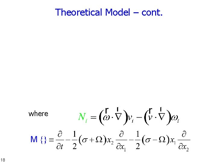
Theoretical Model – cont. where 18

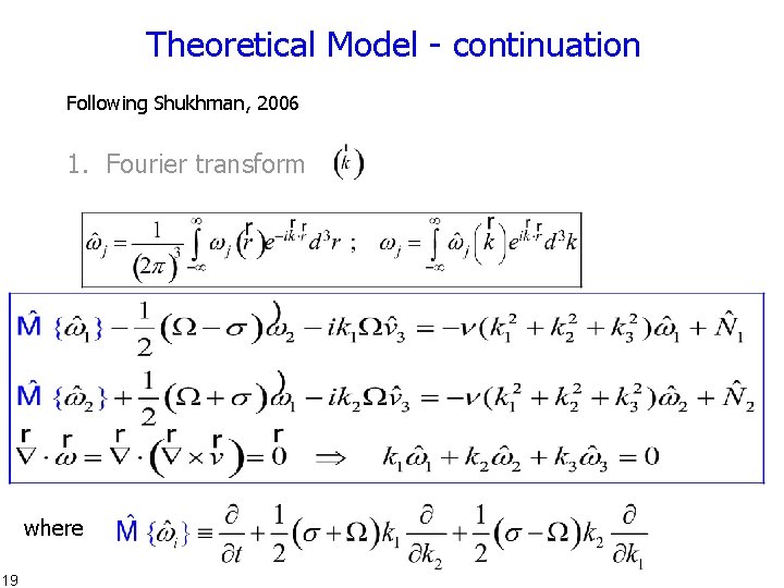
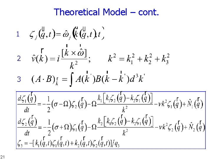
Theoretical Model - continuation Following Shukhman, 2006 1. Fourier transform where 19

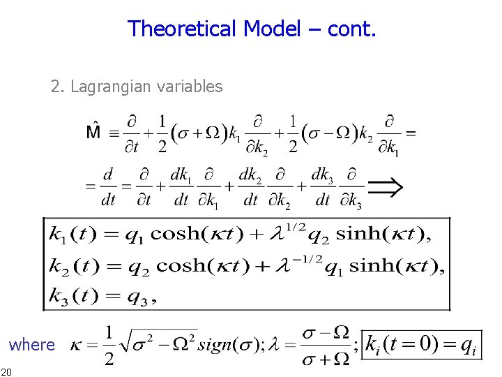
Theoretical Model – cont. 2. Lagrangian variables where 20

Theoretical Model – cont. 1 2 3 21

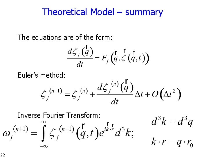
Theoretical Model – summary The equations are of the form: Euler’s method: Inverse Fourier Transform: 22

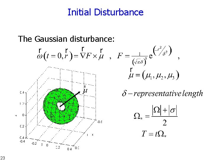
Initial Disturbance The Gaussian disturbance: 23

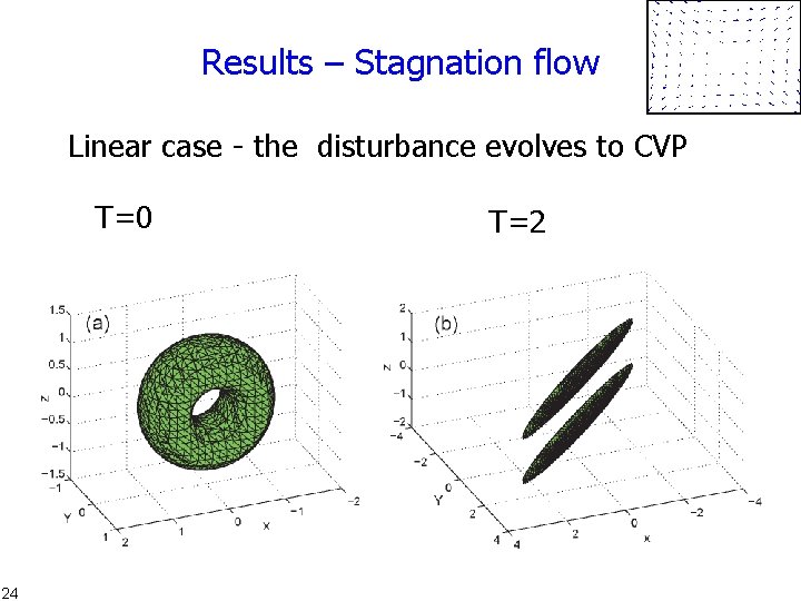
Results – Stagnation flow Linear case - the disturbance evolves to CVP T=0 24 T=2

Results – Stagnation flow Linear case – comparison to the analytical solution T=1, 25 Ω=0, σ=-80 1/sec ( Leonard, 2000 )

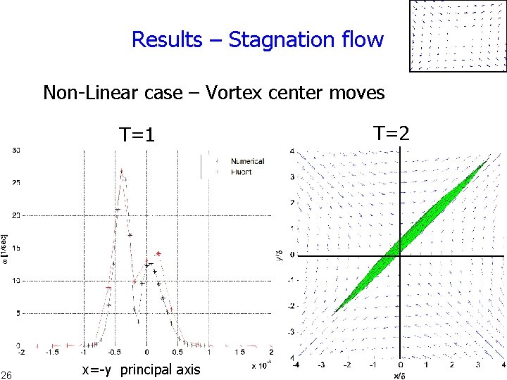
Results – Stagnation flow Non-Linear case – Vortex center moves T=1 26 x=-y principal axis T=2

Results – Couette flow Linear case – comparison to the analytical solution T=1, 27 Ω=σ=-40 1/sec

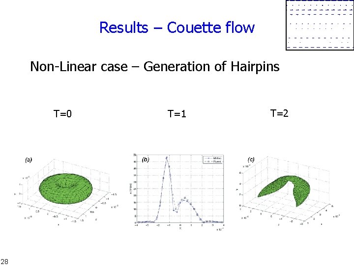
Results – Couette flow Non-Linear case – Generation of Hairpins T=0 28 T=1 T=2

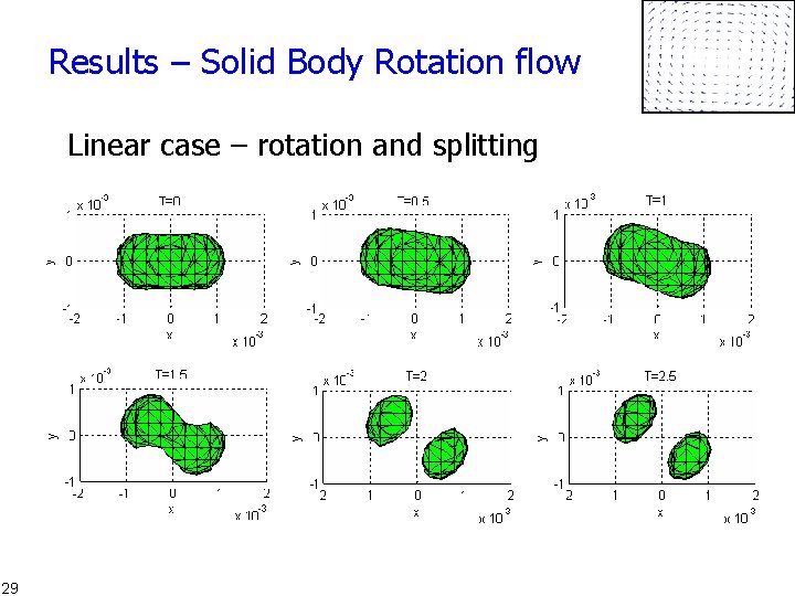
Results – Solid Body Rotation flow Linear case – rotation and splitting 29

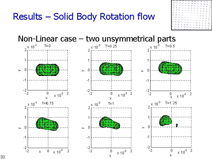
Results – Solid Body Rotation flow Non-Linear case – two unsymmetrical parts 30

Conclusions • An analytical based solution method has been developed • The method can solve the interaction between a family of linear shear flows and any localized disturbance • The solution is carried out using Lagrangian variables in Fourier space which is convenient and enables fast computations Localized Disturbance + Linear Shear Flow Thank You 31 = CVP Hairpins