Lesson 3 2 LeastSquares Regression 5 Minute Check

Lesson 3 - 2 Least-Squares Regression

5 -Minute Check on Section 1 Part 2 1. Describe each scatterplot Positive Linear Strong maybe cluster 2. Identify the explanatory and response variables A study observes a large group of people over a 10 -year period. The goal is to see if overweight and obese people are more likely to die during the study than people who weigh less. Such studies can be misleading because obese people are more likely to be inactive and poor. 3. Could we conclude that increase weight causes greater risk of dying if the study reveals a strong positive correlation? Click the mouse button or press the Space Bar to display the answers.

Objectives • Interpret the slope and y-intercept of a least-squares regression line • Use the least-squares regression line to predict y for a given x • Explain the dangers of extrapolation • Calculate and interpret residuals • Explain the concept of least-squares • Use technology to find a leas-squares regression line • Find the slope and intercept of the least-squares regression line from the means and standard deviations of x and y and their correlation

Objectives • Construct and interpret residual plots to assess if linear model is appropriate • Use the standard deviation of the residuals to assess how well the line fits the data • Use r² to assess how well the line fits the data • Identify the equation of a least-squares regression line from computer output • Explain why association doesn’t imply causation • Recognize how the slope, y-intercept, standard deviation of the residuals and r² are influenced by extreme observations

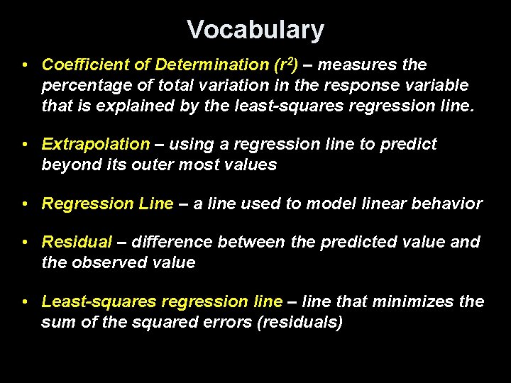
Vocabulary • Coefficient of Determination (r 2) – measures the percentage of total variation in the response variable that is explained by the least-squares regression line. • Extrapolation – using a regression line to predict beyond its outer most values • Regression Line – a line used to model linear behavior • Residual – difference between the predicted value and the observed value • Least-squares regression line – line that minimizes the sum of the squared errors (residuals)

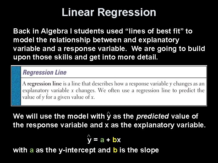
Linear Regression Back in Algebra I students used “lines of best fit” to model the relationship between and explanatory variable and a response variable. We are going to build upon those skills and get into more detail. We will use the model with y as the predicted value of the response variable and x as the explanatory variable. y = a + bx with a as the y-intercept and b is the slope

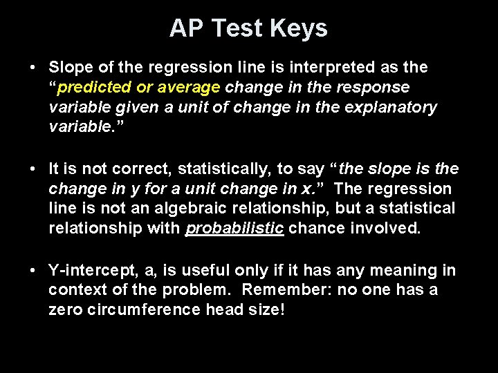
AP Test Keys • Slope of the regression line is interpreted as the “predicted or average change in the response variable given a unit of change in the explanatory variable. ” • It is not correct, statistically, to say “the slope is the change in y for a unit change in x. ” The regression line is not an algebraic relationship, but a statistical relationship with probabilistic chance involved. • Y-intercept, a, is useful only if it has any meaning in context of the problem. Remember: no one has a zero circumference head size!

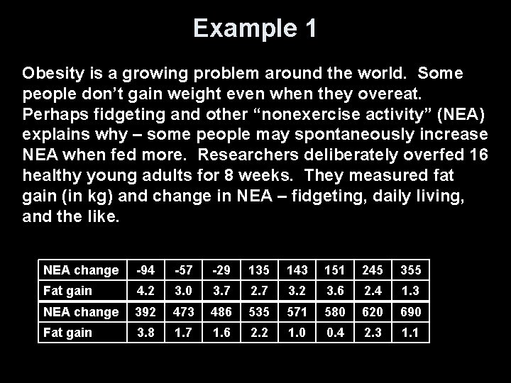
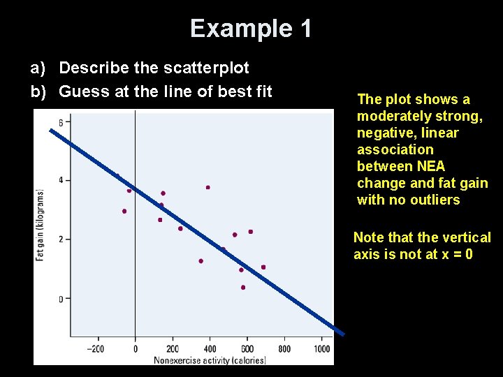
Example 1 Obesity is a growing problem around the world. Some people don’t gain weight even when they overeat. Perhaps fidgeting and other “nonexercise activity” (NEA) explains why – some people may spontaneously increase NEA when fed more. Researchers deliberately overfed 16 healthy young adults for 8 weeks. They measured fat gain (in kg) and change in NEA – fidgeting, daily living, and the like. NEA change -94 -57 -29 135 143 151 245 355 Fat gain 4. 2 3. 0 3. 7 2. 7 3. 2 3. 6 2. 4 1. 3 NEA change 392 473 486 535 571 580 620 690 Fat gain 3. 8 1. 7 1. 6 2. 2 1. 0 0. 4 2. 3 1. 1

Example 1 a) Describe the scatterplot b) Guess at the line of best fit The plot shows a moderately strong, negative, linear association between NEA change and fat gain with no outliers Note that the vertical axis is not at x = 0

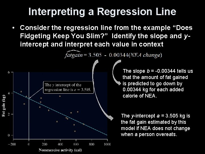
Interpreting a Regression Line • Consider the regression line from the example “Does Fidgeting Keep You Slim? ” Identify the slope and yintercept and interpret each value in context The slope b = -0. 00344 tells us that the amount of fat gained is predicted to go down by 0. 00344 kg for each added calorie of NEA. The y-intercept a = 3. 505 kg is the fat gain estimated by this model if NEA does not change when a person overeats.

Prediction and Extrapolation • Regression lines can be used to predict a response value (y) for a specific explanatory value (x) • Extrapolation, prediction beyond the range of x values in the model, can be very inaccurate and should be done only with noted caution • Extrapolation near the extreme x values generally will be less inaccurate than those done with values farther away from the extreme x values • Note: you can’t say how important a relationship is by looking at the size of the regression slope

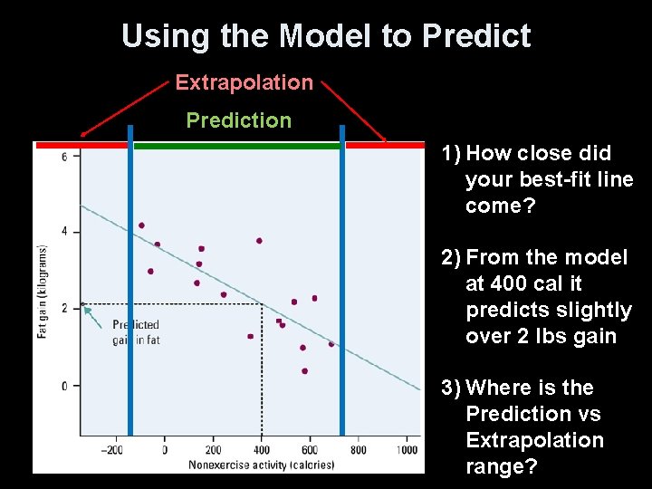
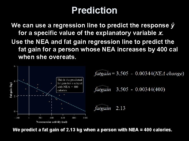
Using the Model to Predict Extrapolation Prediction 1) How close did your best-fit line come? 2) From the model at 400 cal it predicts slightly over 2 lbs gain 3) Where is the Prediction vs Extrapolation range?

Prediction We can use a regression line to predict the response ŷ for a specific value of the explanatory variable x. Use the NEA and fat gain regression line to predict the fat gain for a person whose NEA increases by 400 cal when she overeats. We predict a fat gain of 2. 13 kg when a person with NEA = 400 calories.

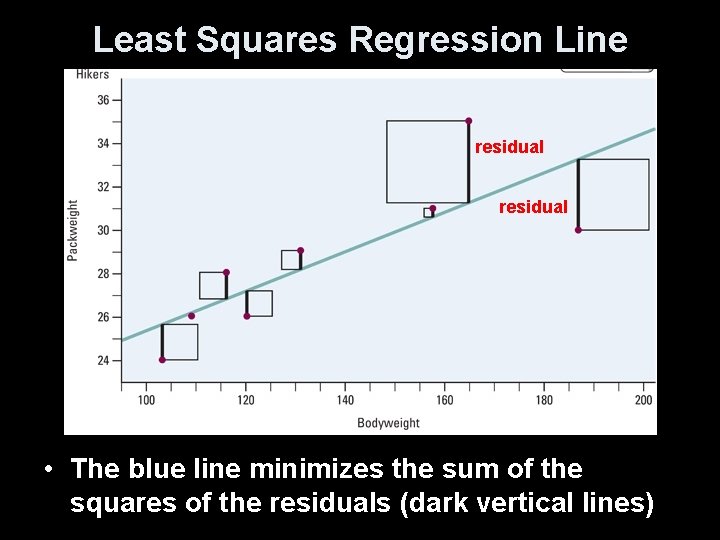
Regression Lines • A good regression line makes the vertical distances of the points from the line (also known as residuals) as small as possible • Residual = Observed - Predicted • The least squares regression line of y on x is the line that makes the sum of the squared residuals as small as possible

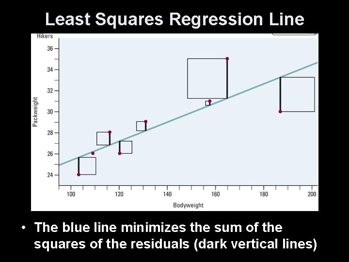
Least Squares Regression Line • The blue line minimizes the sum of the squares of the residuals (dark vertical lines)

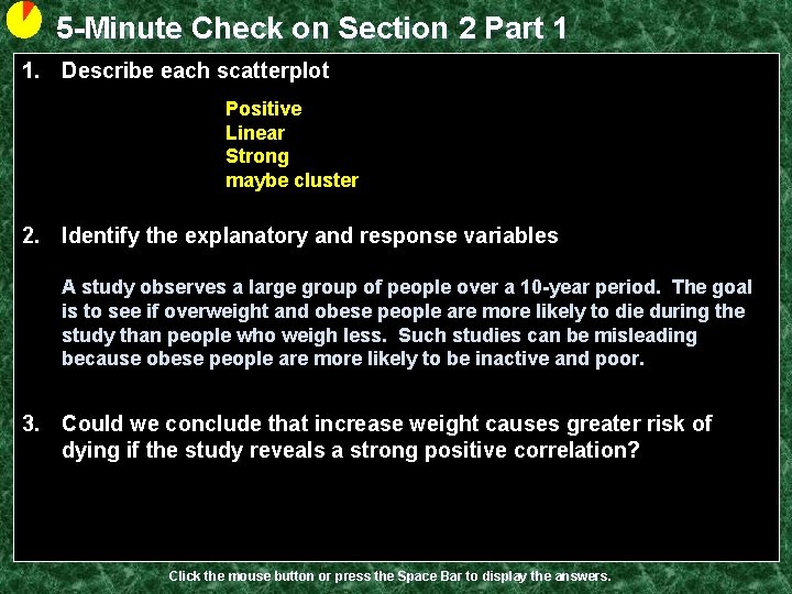
5 -Minute Check on Section 2 Part 1 1. Describe each scatterplot Positive Linear Strong maybe cluster 2. Identify the explanatory and response variables A study observes a large group of people over a 10 -year period. The goal is to see if overweight and obese people are more likely to die during the study than people who weigh less. Such studies can be misleading because obese people are more likely to be inactive and poor. 3. Could we conclude that increase weight causes greater risk of dying if the study reveals a strong positive correlation? Click the mouse button or press the Space Bar to display the answers.

Least Squares Regression Line residual • The blue line minimizes the sum of the squares of the residuals (dark vertical lines)

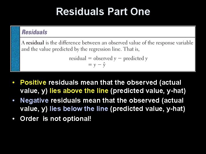
Residuals Part One • Positive residuals mean that the observed (actual value, y) lies above the line (predicted value, y-hat) • Negative residuals mean that the observed (actual value, y) lies below the line (predicted value, y-hat) • Order is not optional!

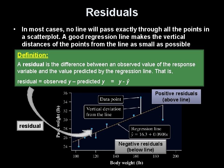
Residuals • In most cases, no line will pass exactly through all the points in a scatterplot. A good regression line makes the vertical distances of the points from the line as small as possible Definition: A residual is the difference between an observed value of the response variable and the value predicted by the regression line. That is, residual = observed y – predicted y = y-ŷ Positive residuals (above line) residual Negative residuals (below line)

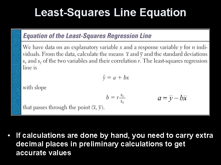
Least-Squares Line Equation • If calculations are done by hand, you need to carry extra decimal places in preliminary calculations to get accurate values

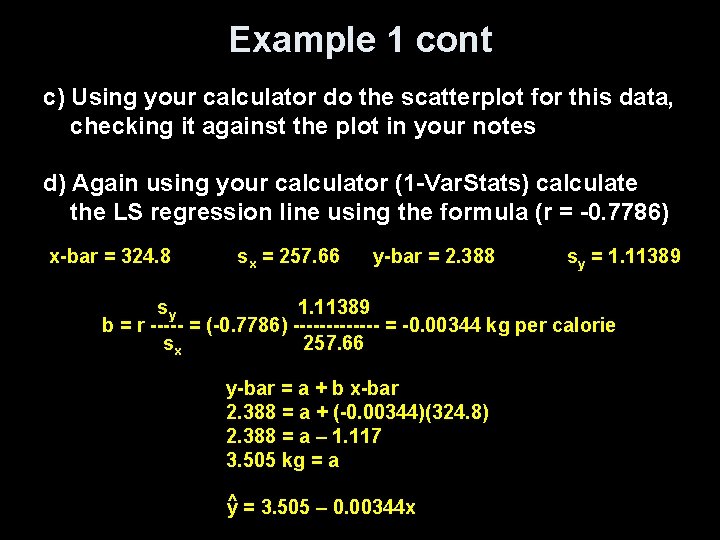
Example 1 cont c) Using your calculator do the scatterplot for this data, checking it against the plot in your notes d) Again using your calculator (1 -Var. Stats) calculate the LS regression line using the formula (r = -0. 7786) x-bar = 324. 8 sx = 257. 66 y-bar = 2. 388 sy = 1. 11389 sy 1. 11389 b = r ----- = (-0. 7786) ------- = -0. 00344 kg per calorie sx 257. 66 y-bar = a + b x-bar 2. 388 = a + (-0. 00344)(324. 8) 2. 388 = a – 1. 117 3. 505 kg = a ^ y = 3. 505 – 0. 00344 x

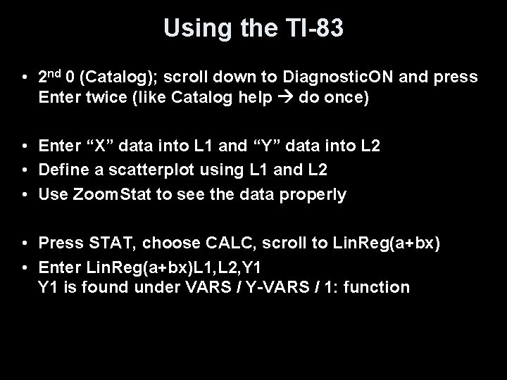
Using the TI-83 • 2 nd 0 (Catalog); scroll down to Diagnostic. ON and press Enter twice (like Catalog help do once) • Enter “X” data into L 1 and “Y” data into L 2 • Define a scatterplot using L 1 and L 2 • Use Zoom. Stat to see the data properly • Press STAT, choose CALC, scroll to Lin. Reg(a+bx) • Enter Lin. Reg(a+bx)L 1, L 2, Y 1 is found under VARS / Y-VARS / 1: function

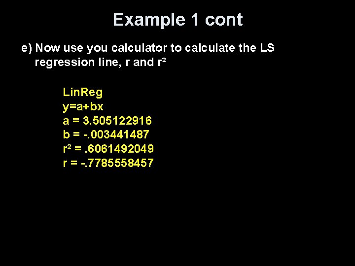
Example 1 cont e) Now use you calculator to calculate the LS regression line, r and r² Lin. Reg y=a+bx a = 3. 505122916 b = -. 003441487 r² =. 6061492049 r = -. 7785558457

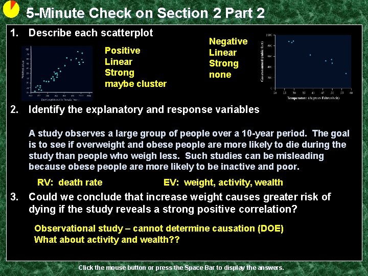
5 -Minute Check on Section 2 Part 2 1. Describe each scatterplot Positive Linear Strong maybe cluster Negative Linear Strong none 2. Identify the explanatory and response variables A study observes a large group of people over a 10 -year period. The goal is to see if overweight and obese people are more likely to die during the study than people who weigh less. Such studies can be misleading because obese people are more likely to be inactive and poor. RV: death rate EV: weight, activity, wealth 3. Could we conclude that increase weight causes greater risk of dying if the study reveals a strong positive correlation? Observational study – cannot determine causation (DOE) What about activity and wealth? ? Click the mouse button or press the Space Bar to display the answers.

Residuals Part Two • The sum of the least-squares residuals is always zero • Residual plots helps assess how well the line describes the data • A good fit has – no discernable pattern to the residuals – and the residuals should be relatively small in size • A poor fit violates one of the above – Discernable patterns: Curved residual plot Increasing / decreasing spread in residual plot

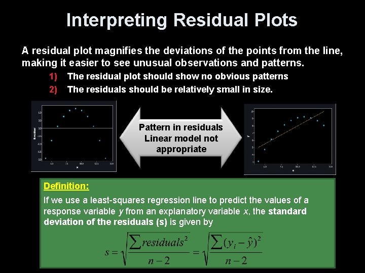
Interpreting Residual Plots A residual plot magnifies the deviations of the points from the line, making it easier to see unusual observations and patterns. 1) 2) The residual plot should show no obvious patterns The residuals should be relatively small in size. Pattern in residuals Linear model not appropriate Definition: If we use a least-squares regression line to predict the values of a response variable y from an explanatory variable x, the standard deviation of the residuals (s) is given by

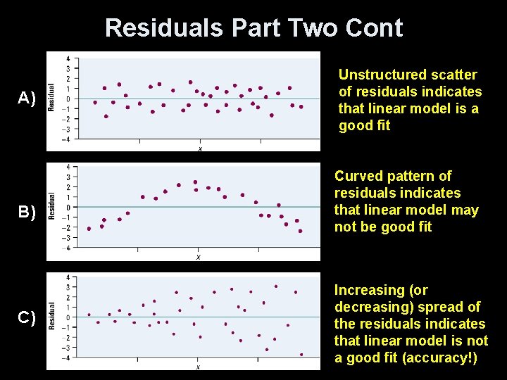
Residuals Part Two Cont A) B) C) Unstructured scatter of residuals indicates that linear model is a good fit Curved pattern of residuals indicates that linear model may not be good fit Increasing (or decreasing) spread of the residuals indicates that linear model is not a good fit (accuracy!)

Residuals Using the TI-83 • After getting the scatterplot (plot 1) and the LS regression line as before • • Define L 3 = Y 1(L 1) [remember how we got Y 1!!] Define L 4 = L 2 – L 3 [actual – predicted] Turn off Plot 1 and deselect the regression eqn (Y=) With Plot 2, plot L 1 as x and L 4 as y • Use 1 -Var. Stat L 4 to find sum of residuals squared Residuals are a calculated list in your list data set after you have run a regression model.

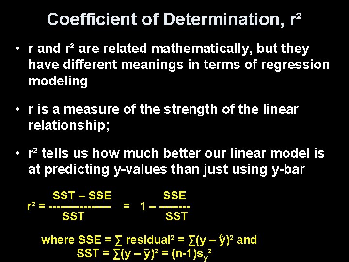
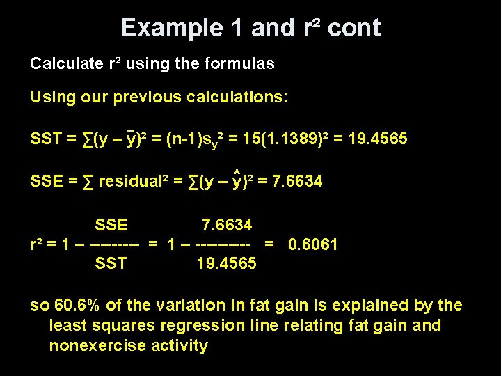
Coefficient of Determination, r² • r and r² are related mathematically, but they have different meanings in terms of regression modeling • r is a measure of the strength of the linear relationship; • r² tells us how much better our linear model is at predicting y-values than just using y-bar SST – SSE r² = --------SST SSE = 1 – -------SST ^ where SSE = ∑ residual² = ∑(y – y)² and _ SST = ∑(y – y)² = (n-1)sy²

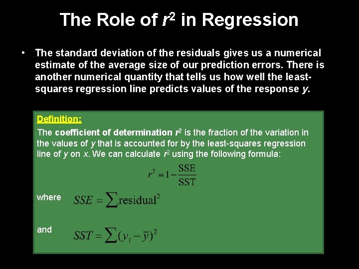
The Role of r 2 in Regression • The standard deviation of the residuals gives us a numerical estimate of the average size of our prediction errors. There is another numerical quantity that tells us how well the leastsquares regression line predicts values of the response y. Definition: The coefficient of determination r 2 is the fraction of the variation in the values of y that is accounted for by the least-squares regression line of y on x. We can calculate r 2 using the following formula: where and

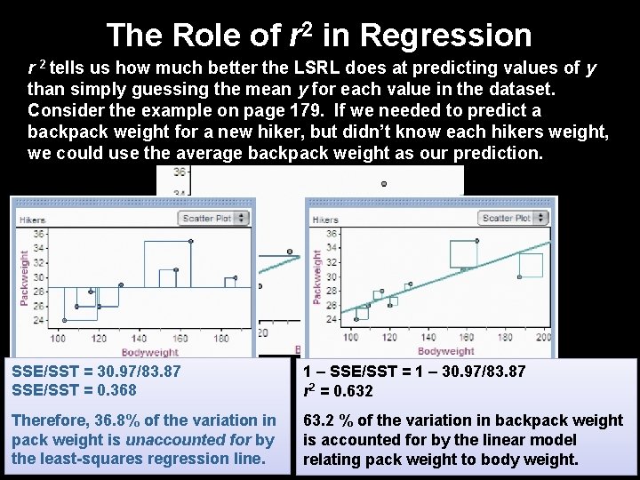
The Role of r 2 in Regression r 2 tells us how much better the LSRL does at predicting values of y than simply guessing the mean y for each value in the dataset. Consider the example on page 179. If we needed to predict a backpack weight for a new hiker, but didn’t know each hikers weight, we could use the average backpack weight as our prediction. SSE/SST = 30. 97/83. 87 SSE/SST = 0. 368 If we use the mean backpack Therefore, 36. 8% of the variation weight as our prediction, the sum in pack is unaccounted for by of theweight squared residuals is 83. 87. the least-squares regression line. SST = 83. 87 1 – SSE/SST = 1 – 30. 97/83. 87 r 2 = 0. 632 If we use the LSRL to make our 63. 2 % of the variation in backpack weight predictions, the sum of the is accounted for by the linear model squared residuals is 30. 90. relating pack weight to body weight. SSE = 30. 90

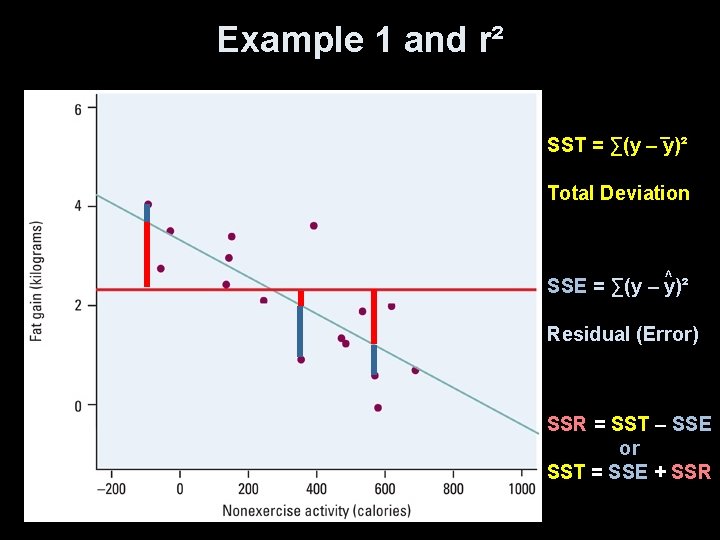
Example 1 and r² _ SST = ∑(y – y)² Total Deviation ^ SSE = ∑(y – y)² Residual (Error) SSR = SST – SSE or SST = SSE + SSR

Example 1 and r² cont Calculate r² using the formulas Using our previous calculations: _ SST = ∑(y – y)² = (n-1)sy² = 15(1. 1389)² = 19. 4565 ^ SSE = ∑ residual² = ∑(y – y)² = 7. 6634 SSE 7. 6634 r² = 1 – ---------- = 0. 6061 SST 19. 4565 so 60. 6% of the variation in fat gain is explained by the least squares regression line relating fat gain and nonexercise activity

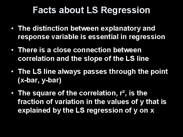
Facts about LS Regression • The distinction between explanatory and response variable is essential in regression • There is a close connection between correlation and the slope of the LS line • The LS line always passes through the point (x-bar, y-bar) • The square of the correlation, r², is the fraction of variation in the values of y that is explained by the LS regression of y on x

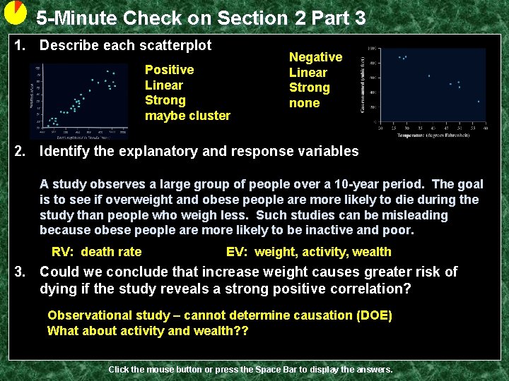
5 -Minute Check on Section 2 Part 3 1. Describe each scatterplot Positive Linear Strong maybe cluster Negative Linear Strong none 2. Identify the explanatory and response variables A study observes a large group of people over a 10 -year period. The goal is to see if overweight and obese people are more likely to die during the study than people who weigh less. Such studies can be misleading because obese people are more likely to be inactive and poor. RV: death rate EV: weight, activity, wealth 3. Could we conclude that increase weight causes greater risk of dying if the study reveals a strong positive correlation? Observational study – cannot determine causation (DOE) What about activity and wealth? ? Click the mouse button or press the Space Bar to display the answers.

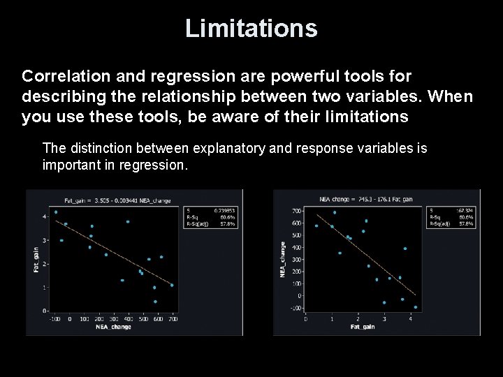
Limitations Correlation and regression are powerful tools for describing the relationship between two variables. When you use these tools, be aware of their limitations The distinction between explanatory and response variables is important in regression.

Limitations • Correlation and regression describe only linear relationships • Extrapolation (using model outside range of the data) often produces unreliable predications • Correlation and least-squares regression lines are not resistant.

Outliers vs Influential Observation • Outlier is an observation that lies outside the overall pattern of the other observations – Outliers in the Y direction will have large residuals. but may not influence the slope of the regression line – Outliers in the X direction are often influential observations • Influential observation is one that if by removing it, it would markedly change the result of the regression calculation

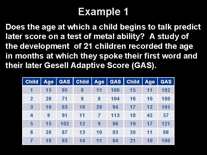
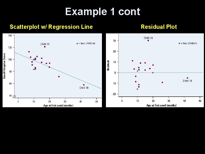
Example 1 Does the age at which a child begins to talk predict later score on a test of metal ability? A study of the development of 21 children recorded the age in months at which they spoke their first word and their later Gesell Adaptive Score (GAS). Child Age GAS 1 15 95 8 11 100 15 11 102 2 26 71 9 8 104 16 10 100 3 10 83 10 20 94 17 12 105 4 9 91 11 7 113 18 42 57 5 15 102 12 9 96 19 17 121 6 20 87 13 10 83 20 11 86 7 18 93 14 11 84 21 10 100

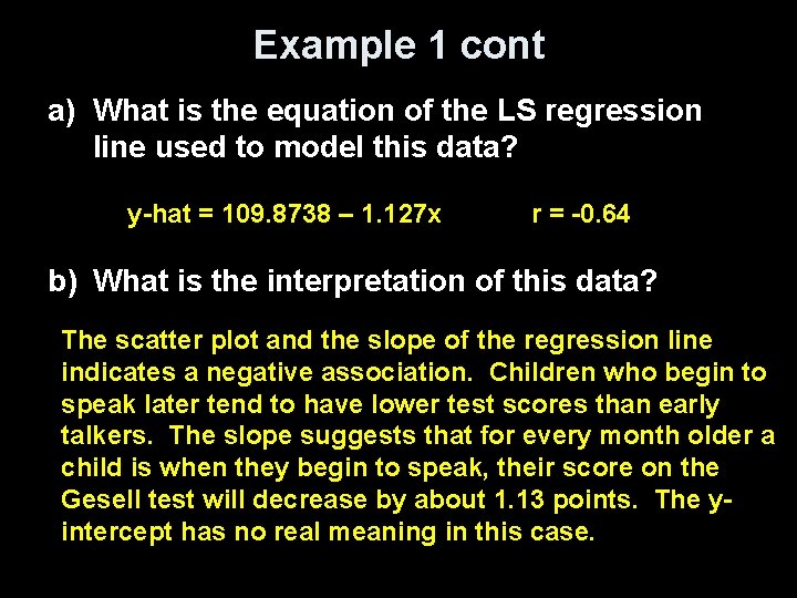
Example 1 cont a) What is the equation of the LS regression line used to model this data? y-hat = 109. 8738 – 1. 127 x r = -0. 64 b) What is the interpretation of this data? The scatter plot and the slope of the regression line indicates a negative association. Children who begin to speak later tend to have lower test scores than early talkers. The slope suggests that for every month older a child is when they begin to speak, their score on the Gesell test will decrease by about 1. 13 points. The yintercept has no real meaning in this case.

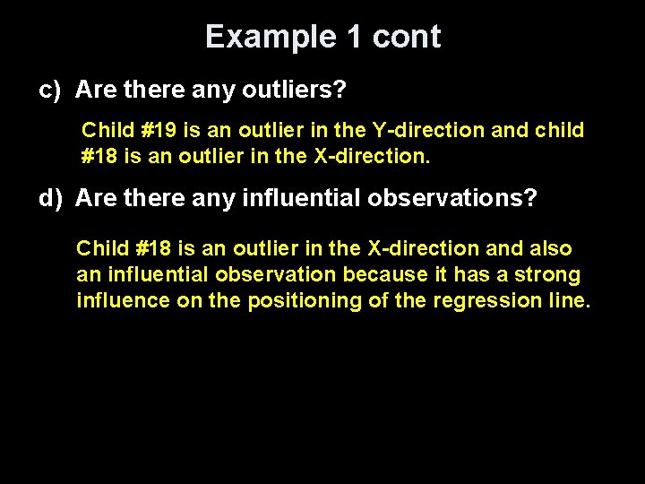
Example 1 cont c) Are there any outliers? Child #19 is an outlier in the Y-direction and child #18 is an outlier in the X-direction. d) Are there any influential observations? Child #18 is an outlier in the X-direction and also an influential observation because it has a strong influence on the positioning of the regression line.

Example 1 cont Scatterplot w/ Regression Line Residual Plot

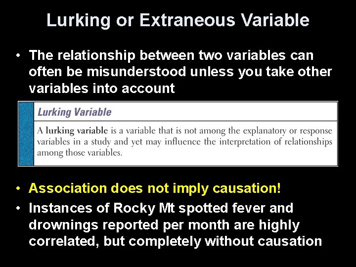
Lurking or Extraneous Variable • The relationship between two variables can often be misunderstood unless you take other variables into account • Association does not imply causation! • Instances of Rocky Mt spotted fever and drownings reported per month are highly correlated, but completely without causation

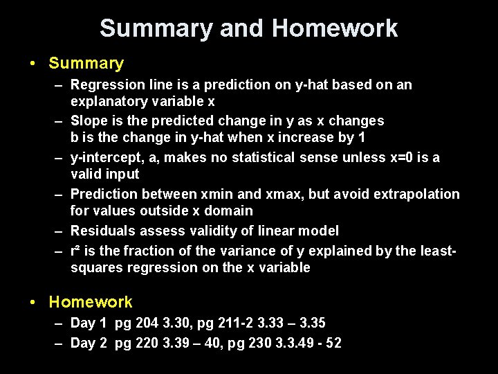
Summary and Homework • Summary – Regression line is a prediction on y-hat based on an explanatory variable x – Slope is the predicted change in y as x changes b is the change in y-hat when x increase by 1 – y-intercept, a, makes no statistical sense unless x=0 is a valid input – Prediction between xmin and xmax, but avoid extrapolation for values outside x domain – Residuals assess validity of linear model – r² is the fraction of the variance of y explained by the leastsquares regression on the x variable • Homework – Day 1 pg 204 3. 30, pg 211 -2 3. 33 – 3. 35 – Day 2 pg 220 3. 39 – 40, pg 230 3. 3. 49 - 52