LECTURE 7 THE CAPM Asset Pricing and Portfolio

LECTURE 7 : THE CAPM (Asset Pricing and Portfolio Theory)

THE CAPM Quantitative Asset Pricing Dirk Nitzsche (E-mail : d. nitzsche@city. ac. uk)

Contents The market portfolio n Factor models : The CAPM Equilibrium model for asset pricing (SML) n Performance measures / Risk adjusted rate of return n Using the CAPM to appraise projects n

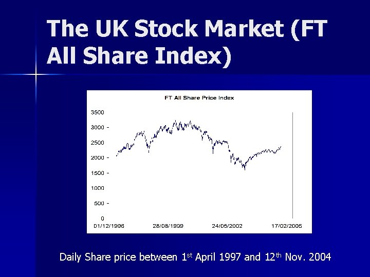
The UK Stock Market (FT All Share Index) Daily Share price between 1 st April 1997 and 12 th Nov. 2004

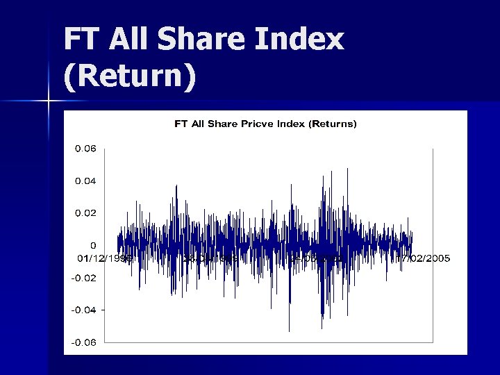
FT All Share Index (Return)

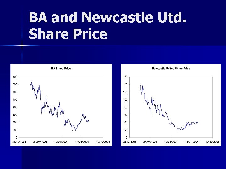
BA and Newcastle Utd. Share Price

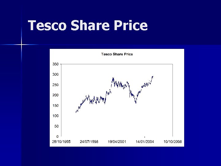
Tesco Share Price

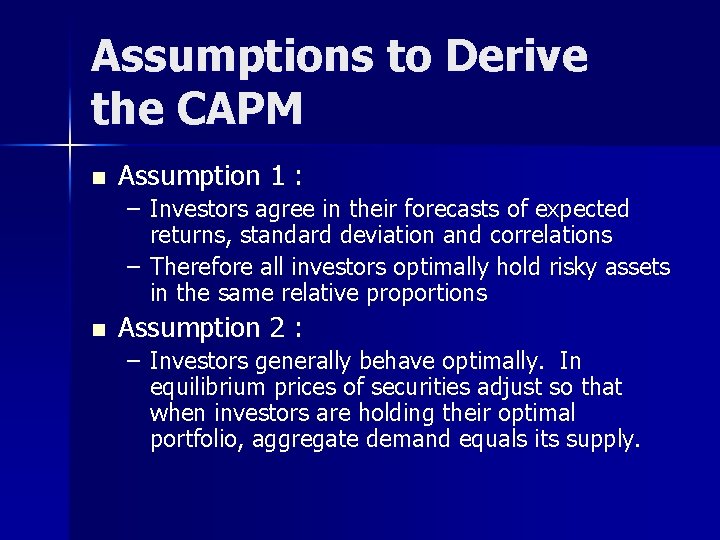
Assumptions to Derive the CAPM n Assumption 1 : – Investors agree in their forecasts of expected returns, standard deviation and correlations – Therefore all investors optimally hold risky assets in the same relative proportions n Assumption 2 : – Investors generally behave optimally. In equilibrium prices of securities adjust so that when investors are holding their optimal portfolio, aggregate demand equals its supply.

The Capital Market Line ERi = rf + [(ERm – rf)/sm] si ER Portfolio M Slope of the CML ERm - rf rf sm Standard deviation

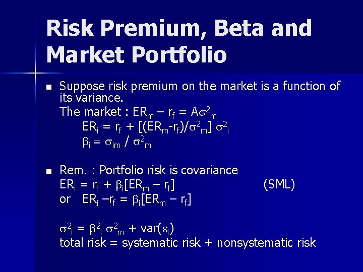
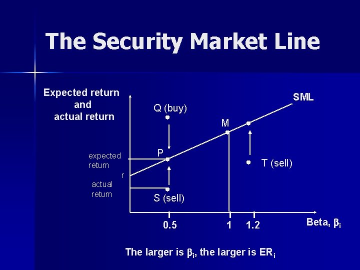
Risk Premium, Beta and Market Portfolio n Suppose risk premium on the market is a function of its variance. The market : ERm – rf = As 2 m ERi = rf + [(ERm-rf)/s 2 m] s 2 i bi sim / s 2 m n Rem. : Portfolio risk is covariance ERi = rf + bi[ERm – rf] or ERi –rf = bi[ERm – rf] (SML) s 2 i = b 2 i s 2 m + var(ei) total risk = systematic risk + nonsystematic risk

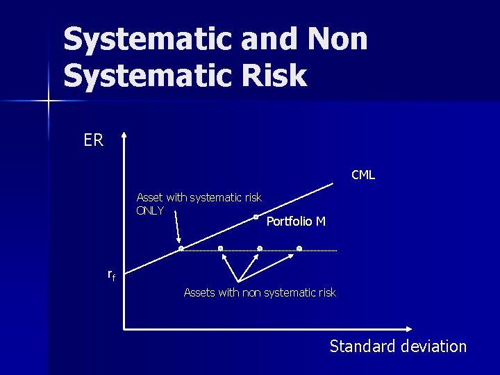
Systematic and Non Systematic Risk ER CML Asset with systematic risk ONLY Portfolio M rf Assets with non systematic risk Standard deviation

The Security Market Line Expected return and actual return SML Q (buy) M P expected return T (sell) r actual return S (sell) 0. 5 1 1. 2 The larger is bi, the larger is ERi Beta, bi

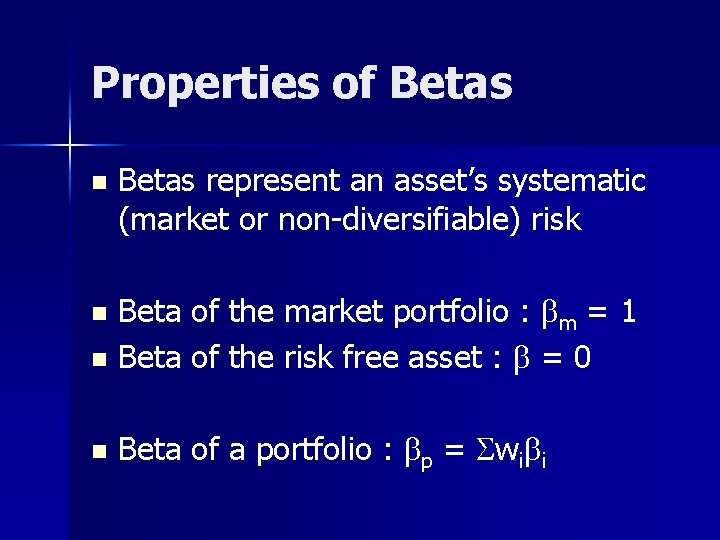
Properties of Betas n Betas represent an asset’s systematic (market or non-diversifiable) risk Beta of the market portfolio : bm = 1 n Beta of the risk free asset : b = 0 n n Beta of a portfolio : bp = Swibi

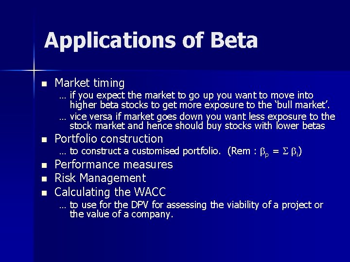
Applications of Beta n Market timing … if you expect the market to go up you want to move into higher beta stocks to get more exposure to the ‘bull market’. … vice versa if market goes down you want less exposure to the stock market and hence should buy stocks with lower betas n Portfolio construction … to construct a customised portfolio. (Rem : bp = S bi) n n n Performance measures Risk Management Calculating the WACC … to use for the DPV for assessing the viability of a project or the value of a company.

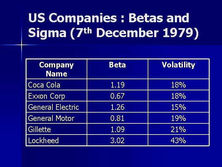
US Companies : Betas and Sigma (7 th December 1979) Company Name Coca Cola Exxon Corp General Electric General Motor Gillette Lockheed Beta Volatility 1. 19 0. 67 18% 1. 26 0. 81 1. 09 3. 02 15% 19% 21% 43%

Performance Measures / Risk Adjusted Rate of Return

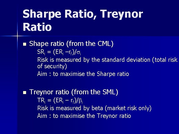
Sharpe Ratio, Treynor Ratio n Shape ratio (from the CML) SRi = (ERi –rf)/si Risk is measured by the standard deviation (total risk of security) Aim : to maximise the Sharpe ratio n Treynor ratio (from the SML) TRi = (ERi – rf)/bi Risk is measured by beta (market risk only) Aim : to maximise the Treynor ratio

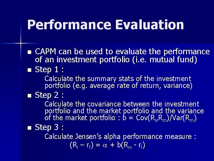
Performance Evaluation n n CAPM can be used to evaluate the performance of an investment portfolio (i. e. mutual fund) Step 1 : Calculate the summary stats of the investment portfolio (e. g. average rate of return, variance) n Step 2 : Calculate the covariance between the investment portfolio and the market portfolio and the variance of the market portfolio : b = Cov(Ri, Rm)/Var(Rm) n Step 3 : Calculate Jensen’s alpha performance measure : (Ri – rf) = a + b(Rm - rf)

Obtaining Beta

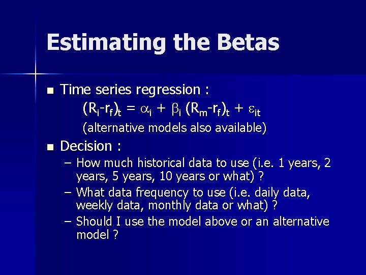
Estimating the Betas n Time series regression : (Ri-rf)t = ai + bi (Rm-rf)t + eit (alternative models also available) n Decision : – How much historical data to use (i. e. 1 years, 2 years, 5 years, 10 years or what) ? – What data frequency to use (i. e. daily data, weekly data, monthly data or what) ? – Should I use the model above or an alternative model ?

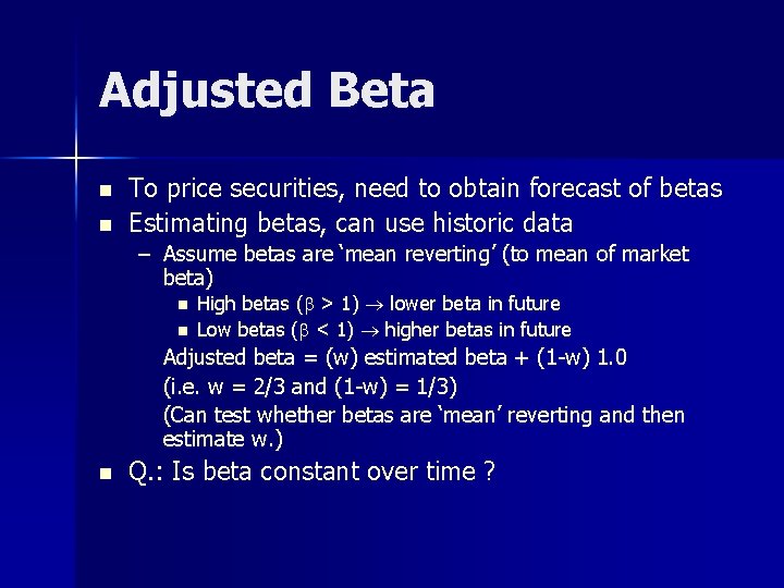
Adjusted Beta n n To price securities, need to obtain forecast of betas Estimating betas, can use historic data – Assume betas are ‘mean reverting’ (to mean of market beta) n n High betas (b > 1) lower beta in future Low betas (b < 1) higher betas in future Adjusted beta = (w) estimated beta + (1 -w) 1. 0 (i. e. w = 2/3 and (1 -w) = 1/3) (Can test whether betas are ‘mean’ reverting and then estimate w. ) n Q. : Is beta constant over time ?

CAPM and Investment Appraisal

CAPM and Investment Appraisal (All Equity Firm) n n n Expected return ERi on equity (calculated from the CAPM formula) is (often) used as the discount rate in a DPV calculation to assess a physical investment project for an all equity financed firm We use ERi because it reflects the riskiness of the firm’s new investment project – provided the ‘new’ investment project has the same ‘business risk’ characteristics as the firm’s existing project. This is because ERi reflects the return required by investors to hold this share as part of their portfolio (of shares) to compensate them, for the (beta-) risk of the firm (i. e. due to covariance with the market return, over the past).

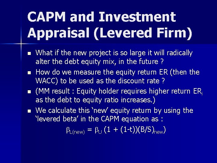
CAPM and Investment Appraisal (Levered Firm) n n What if the new project is so large it will radically alter the debt equity mix, in the future ? How do we measure the equity return ER (then the WACC) to be used as the discount rate ? (MM result : Equity holder requires higher return ERi as the debt to equity ratio increases. ) We calculate this ‘new’ equity return by using the ‘levered beta’ in the CAPM equation as : b. L(new) = b. U (1 + (1 -t))(B/S)new)

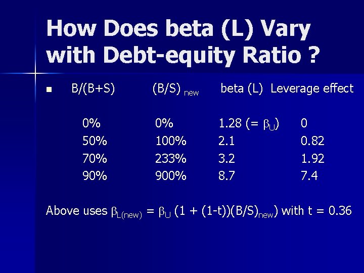
How Does beta (L) Vary with Debt-equity Ratio ? n B/(B+S) 0% 50% 70% 90% (B/S) new beta (L) Leverage effect 0% 100% 233% 900% 1. 28 (= b. U) 2. 1 3. 2 8. 7 0 0. 82 1. 92 7. 4 Above uses b. L(new) = b. U (1 + (1 -t))(B/S)new) with t = 0. 36

How Does beta (L) Vary with Debt-equity Ratio ? (Cont. ) n n n The ‘leverage-beta’ increases with leverage (B/S) and hence so does the required return on equity ERi given by the CAPM and hence the discount rate for cash flows ERi can then be used with the bond yield to calculate WACC, if debt and equity finance is being used for the ‘new’ project. See Cuthbertson and Nitzsche (2001) ‘Investments : Spot and Derivatives Markets’

Variants of the CAPM

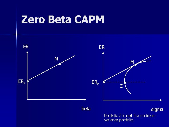
Zero Beta CAPM ER ER M M ERz beta Z sigma Portfolio Z is not the minimum variance portfolio.

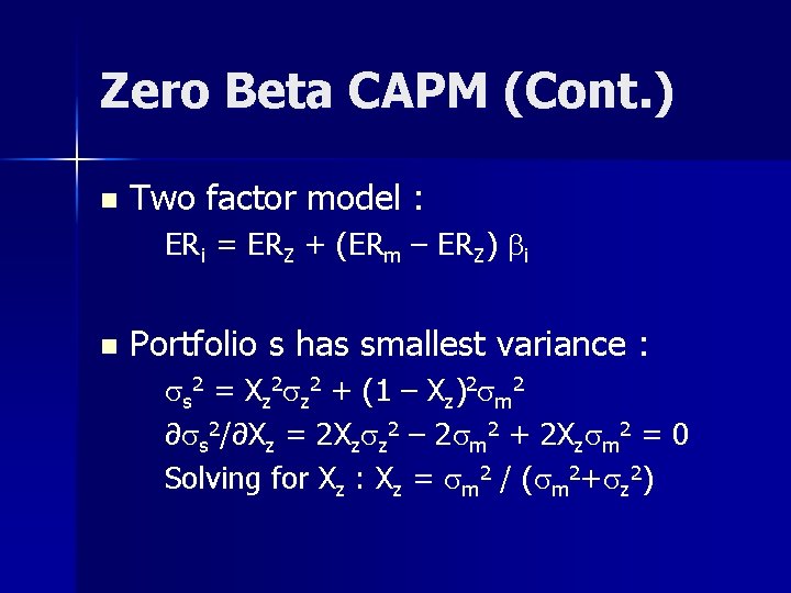
Zero Beta CAPM (Cont. ) n Two factor model : ERi = ERZ + (ERm – ERZ) bi n Portfolio s has smallest variance : ss 2 = Xz 2 sz 2 + (1 – Xz)2 sm 2 ∂ss 2/∂Xz = 2 Xzsz 2 – 2 sm 2 + 2 Xzsm 2 = 0 Solving for Xz : Xz = sm 2 / (sm 2+sz 2)

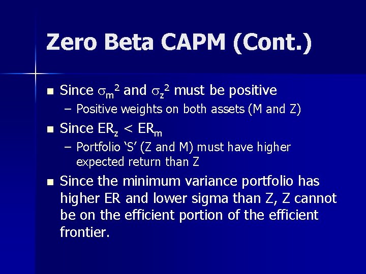
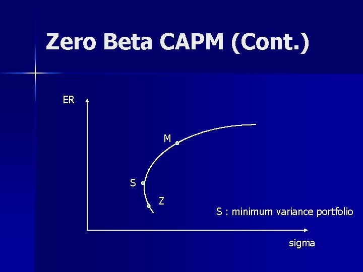
Zero Beta CAPM (Cont. ) n Since sm 2 and sz 2 must be positive – Positive weights on both assets (M and Z) n Since ERz < ERm – Portfolio ‘S’ (Z and M) must have higher expected return than Z n Since the minimum variance portfolio has higher ER and lower sigma than Z, Z cannot be on the efficient portion of the efficient frontier.

Zero Beta CAPM (Cont. ) ER M S Z S : minimum variance portfolio sigma

The Consumption CAPM Different definition of equilibrium in the capital market n Key assumption : n – Investors maximise a multiperiod utility function over lifetime consumption – Homogeneous beliefs about asset characteristics – Infinitely lived population, one consumption good

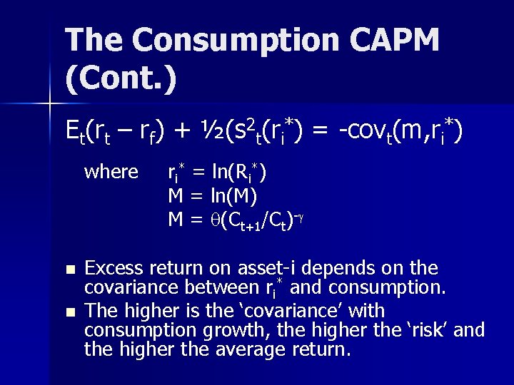
The Consumption CAPM (Cont. ) Et(rt – rf) + ½(s 2 t(ri*) = -covt(m, ri*) where n n ri* = ln(Ri*) M = ln(M) M = q(Ct+1/Ct)-g Excess return on asset-i depends on the covariance between ri* and consumption. The higher is the ‘covariance’ with consumption growth, the higher the ‘risk’ and the higher the average return.

References Cuthbertson, K. and Nitzsche, D. (2004) ‘Quantitative Financial Economics’, Chapters 7 n Cuthbertson, K. and Nitzsche, D. (2001) ‘Investments : Spot and Derivatives Markets’, Chapter 10. 3 n

END OF LECTURE