Investment Analysis and Portfolio Management The Capital Asset

Investment Analysis and Portfolio Management • The Capital Asset Pricing Model (CAPM) – – 5. 6. 2021 Review of Portfolio Theory The Capital Asset Pricing Model Implementing the CAPM F-F 3 Factor Model 1

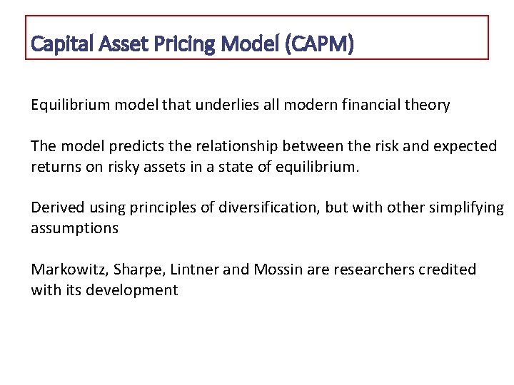
Capital Asset Pricing Model (CAPM) Equilibrium model that underlies all modern financial theory The model predicts the relationship between the risk and expected returns on risky assets in a state of equilibrium. Derived using principles of diversification, but with other simplifying assumptions Markowitz, Sharpe, Lintner and Mossin are researchers credited with its development

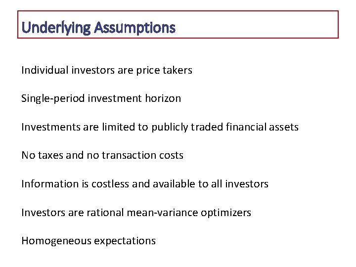
Underlying Assumptions Individual investors are price takers Single-period investment horizon Investments are limited to publicly traded financial assets No taxes and no transaction costs Information is costless and available to all investors Investors are rational mean-variance optimizers Homogeneous expectations

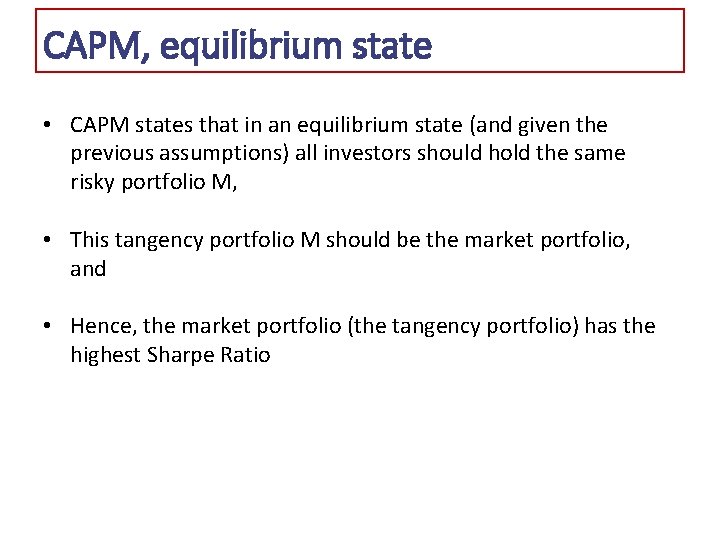
CAPM, equilibrium state • CAPM states that in an equilibrium state (and given the previous assumptions) all investors should hold the same risky portfolio M, • This tangency portfolio M should be the market portfolio, and • Hence, the market portfolio (the tangency portfolio) has the highest Sharpe Ratio

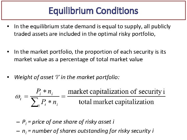
Equilibrium Conditions • In the equilibrium state demand is equal to supply, all publicly traded assets are included in the optimal risky portfolio, • In the market portfolio, the proportion of each security is its market value as a percentage of total market value • Weight of asset ‘i’ in the market portfolio: – Pi = price of one share of risky asset i – ni = number of shares outstanding for risky security i

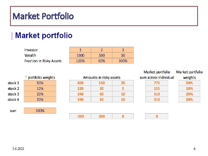
Market Portfolio 5. 6. 2021 6

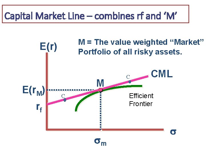
The Capital Market Line (CML) • From the above analysis, the CAPM predicts that the Market Portfolio is the optimal risky portfolio. • The CAL that connects the riskless security and the market portfolio is called the Capital Market Line. • Then, investors should decide how to allocate their wealth between: – The market portfolio, and – A riskless security 5. 6. 2021 7

Capital Market Line – combines rf and ‘M’ M = The value weighted “Market” Portfolio of all risky assets. E(r) E(r. M) M C CML Efficient Frontier C rf sm s

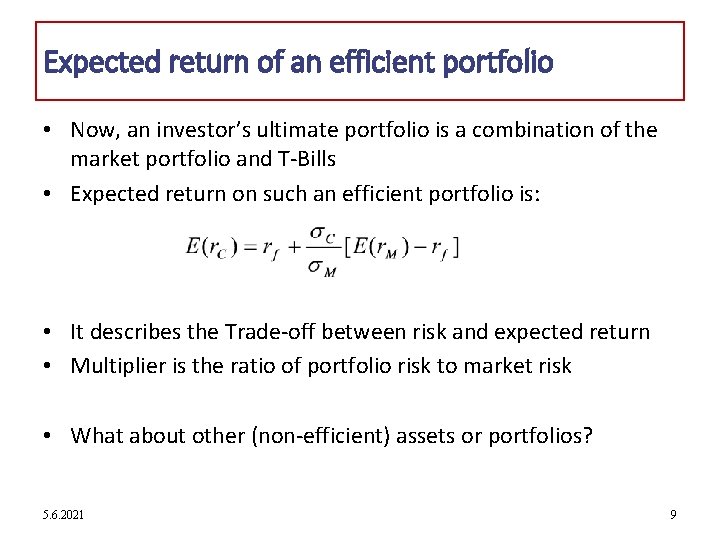
Expected return of an efficient portfolio • Now, an investor’s ultimate portfolio is a combination of the market portfolio and T-Bills • Expected return on such an efficient portfolio is: • It describes the Trade-off between risk and expected return • Multiplier is the ratio of portfolio risk to market risk • What about other (non-efficient) assets or portfolios? 5. 6. 2021 9

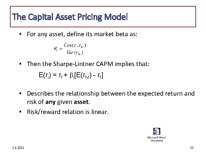
The Capital Asset Pricing Model • For any asset, define its market beta as: • Then the Sharpe-Lintner CAPM implies that: E(ri) = rf + i[E(r. M) - rf] • Describes the relationship between the expected return and risk of any given asset. • Risk/reward relation is linear. 5. 6. 2021 10

Beta • Beta measures sensitivity of stock volatility to market volatility. • The i measures the risk of an asset that we cannot diversify away by combining it with other assets in the market portfolio. • The higher the Beta is for any asset, the higher must be its return. 5. 6. 2021 11

Security Market Line 5. 6. 2021 12

Security Market Line 5. 6. 2021 13

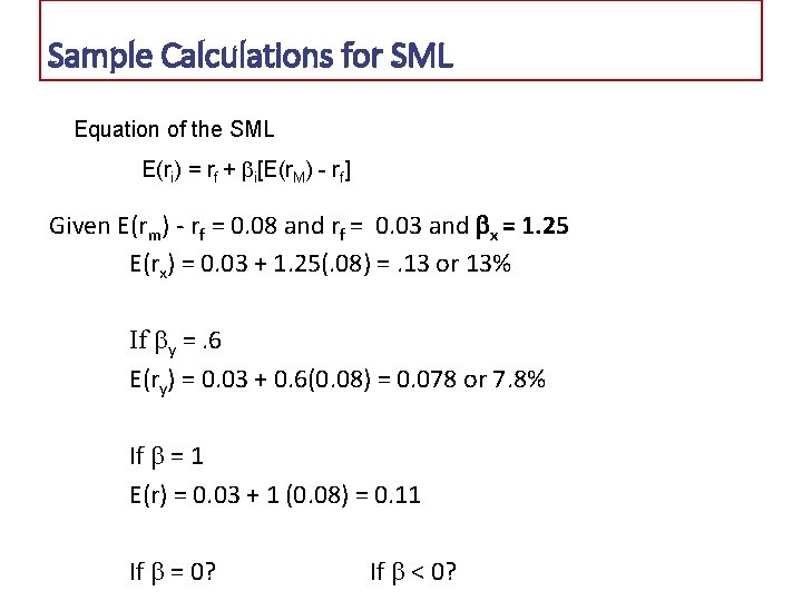
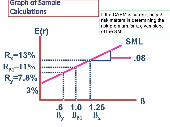
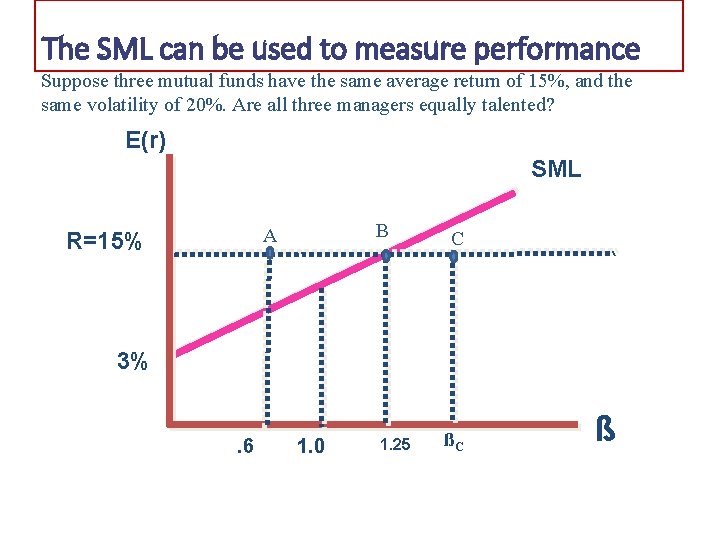
Sample Calculations for SML Equation of the SML E(ri) = rf + i[E(r. M) - rf] Given E(rm) - rf = 0. 08 and rf = 0. 03 and bx = 1. 25 E(rx) = 0. 03 + 1. 25(. 08) =. 13 or 13% If y =. 6 E(ry) = 0. 03 + 0. 6(0. 08) = 0. 078 or 7. 8% If = 1 E(r) = 0. 03 + 1 (0. 08) = 0. 11 If = 0? If < 0?

Graph of Sample Calculations E(r) If the CAPM is correct, only β risk matters in determining the risk premium for a given slope of the SML Rx=13% RM=11% Ry=7. 8% 3% . 08 . 6 1. 0 1. 25 ßy ßM ßx ß

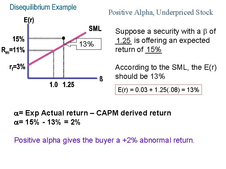
Positive Alpha, Underpriced Stock 13% Suppose a security with a of ____ 1. 25 is offering an expected 15% return of ____ According to the SML, the E(r) should be 13% E(r) = 0. 03 + 1. 25(. 08) = 13% a= Exp Actual return – CAPM derived return a= 15% - 13% = 2% Positive alpha gives the buyer a +2% abnormal return.

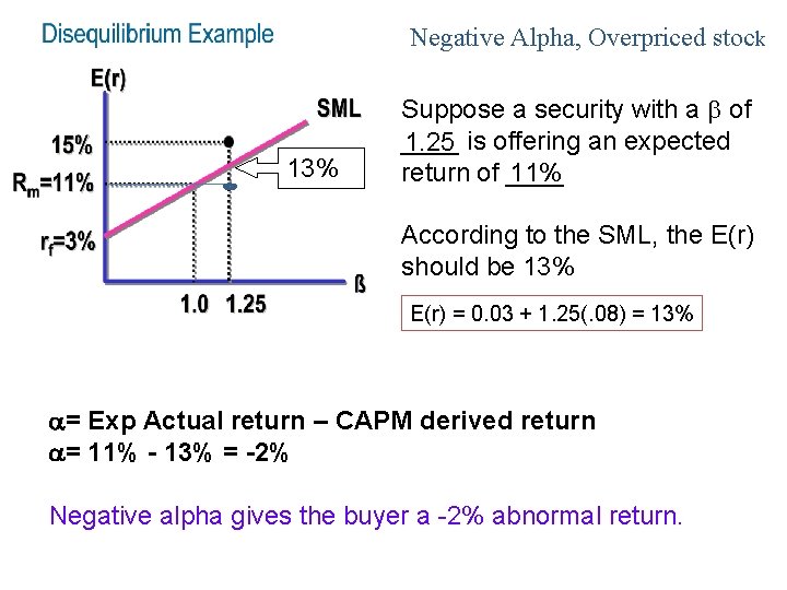
Negative Alpha, Overpriced stock 13% Suppose a security with a of ____ 1. 25 is offering an expected 11% return of ____ According to the SML, the E(r) should be 13% E(r) = 0. 03 + 1. 25(. 08) = 13% a= Exp Actual return – CAPM derived return a= 11% - 13% = -2% Negative alpha gives the buyer a -2% abnormal return.

The SML can be used to measure performance Suppose three mutual funds have the same average return of 15%, and the same volatility of 20%. Are all three managers equally talented? E(r) SML B A R=15% C 3%. 6 1. 0 1. 25 ßC ß

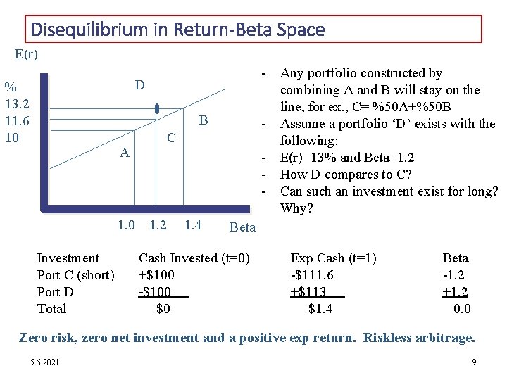
Disequilibrium in Return-Beta Space E(r) - Any portfolio constructed by combining A and B will stay on the line, for ex. , C= %50 A+%50 B - Assume a portfolio ‘D’ exists with the following: - E(r)=13% and Beta=1. 2 - How D compares to C? - Can such an investment exist for long? Why? D % 13. 2 11. 6 10 B A 1. 0 Investment Port C (short) Port D Total C 1. 2 1. 4 Beta Cash Invested (t=0) +$100 -$100 $0 Exp Cash (t=1) -$111. 6 +$113 $1. 4 Beta -1. 2 +1. 2 0. 0 Zero risk, zero net investment and a positive exp return. Riskless arbitrage. 5. 6. 2021 19

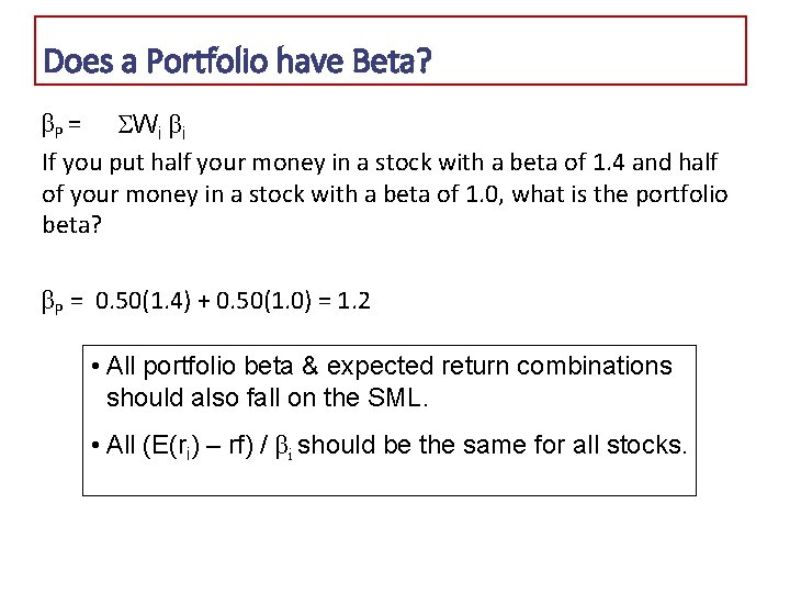
Does a Portfolio have Beta? βP = Wi βi If you put half your money in a stock with a beta of 1. 4 and half of your money in a stock with a beta of 1. 0, what is the portfolio beta? βP = 0. 50(1. 4) + 0. 50(1. 0) = 1. 2 • All portfolio beta & expected return combinations should also fall on the SML. • All (E(ri) – rf) / βi should be the same for all stocks.

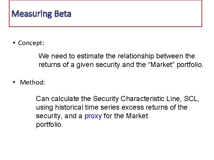
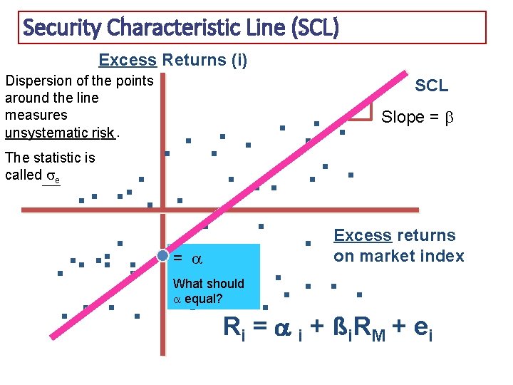
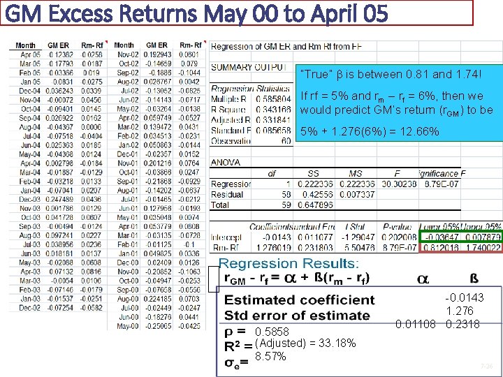
Measuring Beta • Concept: We need to estimate the relationship between the returns of a given security and the “Market” portfolio. • Method: Can calculate the Security Characteristic Line, SCL, using historical time series excess returns of the security, and a proxy for the Market portfolio.

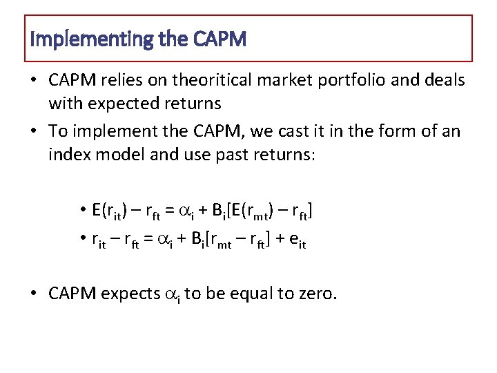
Implementing the CAPM • CAPM relies on theoritical market portfolio and deals with expected returns • To implement the CAPM, we cast it in the form of an index model and use past returns: • E(rit) – rft = i + Bi[E(rmt) – rft] • rit – rft = i + Bi[rmt – rft] + eit • CAPM expects i to be equal to zero.

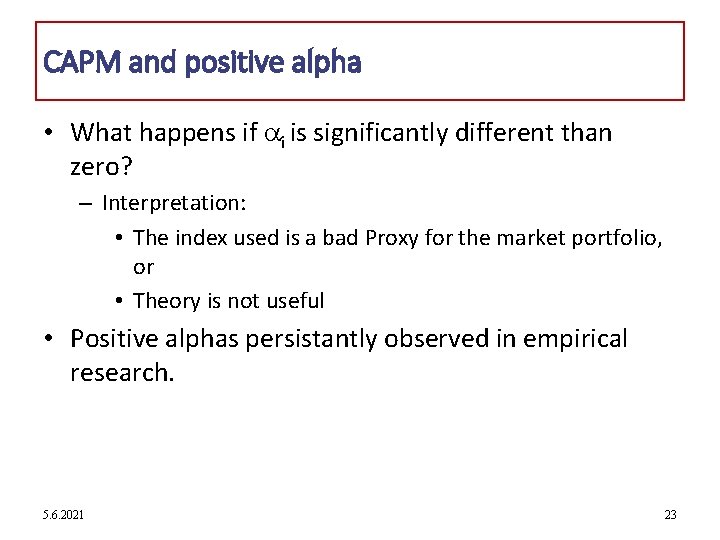
CAPM and positive alpha • What happens if i is significantly different than zero? – Interpretation: • The index used is a bad Proxy for the market portfolio, or • Theory is not useful • Positive alphas persistantly observed in empirical research. 5. 6. 2021 23

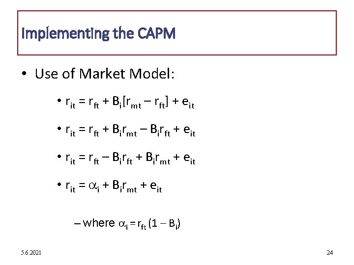
Implementing the CAPM • Use of Market Model: • rit = rft + Bi[rmt – rft] + eit • rit = rft + Birmt – Birft + eit • rit = rft – Birft + Birmt + eit • rit = i + Birmt + eit – where i = rft (1 – Bi) 5. 6. 2021 24

Security Characteristic Line (SCL) Excess Returns (i) Dispersion of the points around the line measures _______. unsystematic risk SCL Slope = . . The statistic is. . called . . . Excess returns. . . on market index. . . = . . R =. a + ß R + e e What should equal? i i i M i

GM Excess Returns May 00 to April 05 “True” is between 0. 81 and 1. 74! If rf = 5% and rm – rf = 6%, then we would predict GM’s return (r. GM) to be 5% + 1. 276(6%) = 12. 66% 0. 5858 (Adjusted) = 33. 18% 8. 57% -0. 0143 1. 276 0. 01108 0. 2318 7 -26

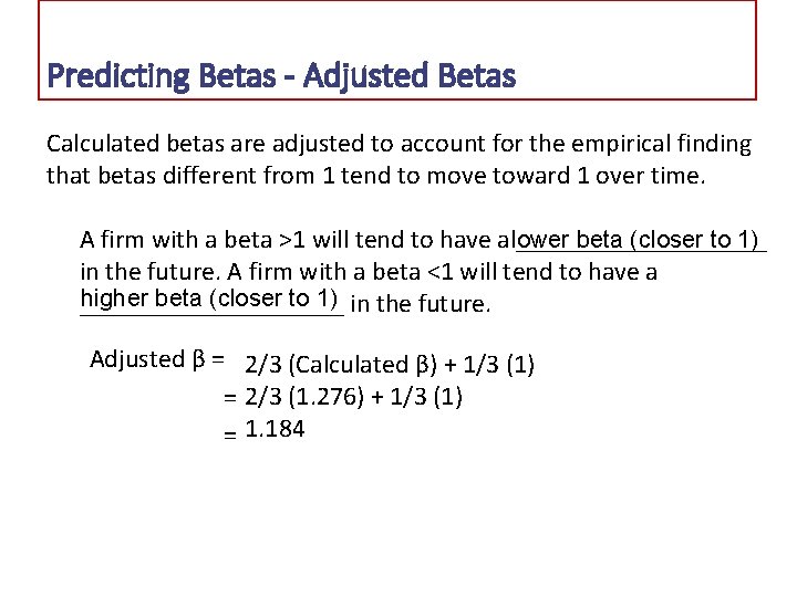
Predicting Betas - Adjusted Betas Calculated betas are adjusted to account for the empirical finding that betas different from 1 tend to move toward 1 over time. beta (closer to 1) A firm with a beta >1 will tend to have a lower __________ in the future. A firm with a beta <1 will tend to have a higher beta (closer to 1) in the future. __________ Adjusted β = 2/3 (Calculated β) + 1/3 (1) = 2/3 (1. 276) + 1/3 (1) = 1. 184

Predictions and applications • Predictions: – CAPM: In market equilibrium, investors are only rewarded for bearing the market risk, • Applications: – Evaluating security returns – Corporate manager: capital budgeting decisions, company valuations – Regulatory commissions: cost of capital for regulated firms (eg. , utilities) – Professional portfolio managers: evaluating security returns and fund performance. 5. 6. 2021 28

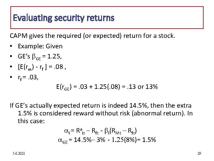
Evaluating security returns CAPM gives the required (or expected) return for a stock. • Example: Given • GE’s GE = 1. 25, • [E(rm) - rf ] =. 08 , • rf =. 03, E(r. GE) =. 03 + 1. 25(. 08) =. 13 or 13% If GE’s actually expected return is indeed 14. 5%, then the extra 1. 5% is considered reward without risk (abnormal return). In this case: i = Rait – Rft - i(RMt – Rft) GE = 14. 5%– 3% - 1. 25(8%)= 1. 5% 5. 6. 2021 29

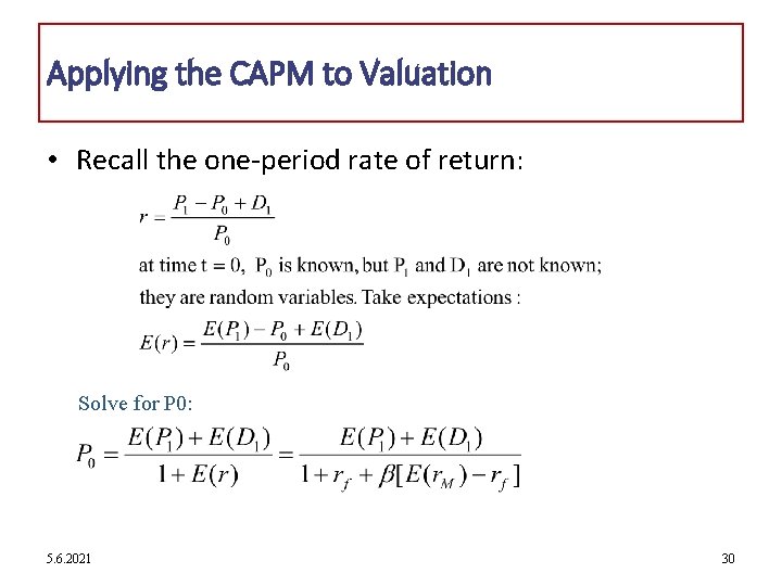
Applying the CAPM to Valuation • Recall the one-period rate of return: Solve for P 0: 5. 6. 2021 30

Example: Stock Valuation using CAPM • E[D 1] = 5, g = 0. 10, rf = 0. 03 • Beta = 1. 5, E[rm – rf] = 0. 075 • E[r] = rf + B[E(rm) – rf) = 0. 03+1. 5(0. 075)= 0. 1425 • Constant growth: 5. 6. 2021 31

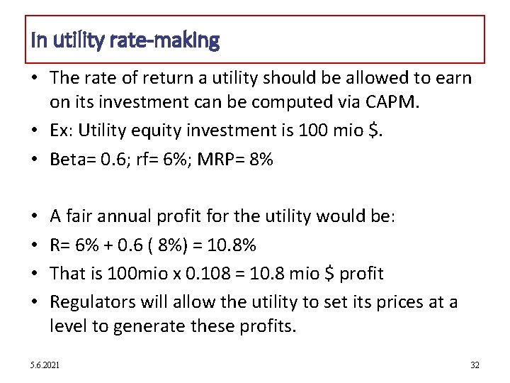
In utility rate-making • The rate of return a utility should be allowed to earn on its investment can be computed via CAPM. • Ex: Utility equity investment is 100 mio $. • Beta= 0. 6; rf= 6%; MRP= 8% • • A fair annual profit for the utility would be: R= 6% + 0. 6 ( 8%) = 10. 8% That is 100 mio x 0. 108 = 10. 8 mio $ profit Regulators will allow the utility to set its prices at a level to generate these profits. 5. 6. 2021 32

Other Applications of CAPM • Market timing: – If Betas are correctly estimated and likely to stay constant in the (near? ) future then you can use betas for market timing. How? • Used in portfolio choice: – If you want to hold a diversified portfolio but one that has a specific beta that you want, you can use the concept of portfolio beta. 5. 6. 2021 33

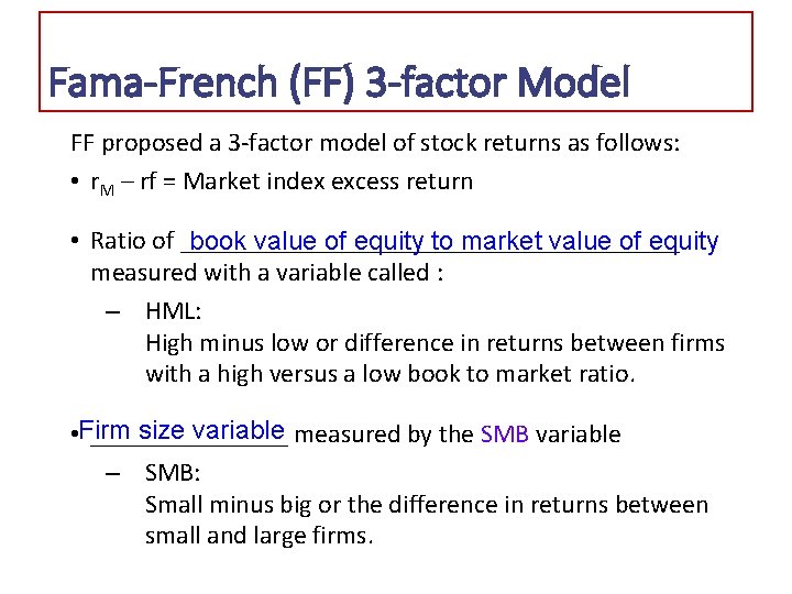
Fama-French (FF) 3 -Factor Model Fama and French noted that stocks of smaller firms and stocks of firms with a high book to market ratio have had higher stock returns than predicted by single factor models. • Problem: Empirical model without a theory • Will the variables continue to have predictive power?

Fama-French (FF) 3 -factor Model FF proposed a 3 -factor model of stock returns as follows: • r. M – rf = Market index excess return • Ratio of ___________________ book value of equity to market value of equity measured with a variable called : – HML: High minus low or difference in returns between firms with a high versus a low book to market ratio. size variable measured by the SMB variable • Firm ________ – SMB: Small minus big or the difference in returns between small and large firms.

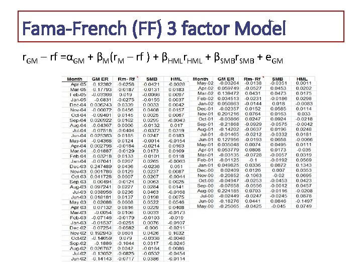
Fama-French (FF) 3 factor Model r. GM – rf =αGM + βM(r. M – rf ) + βHMLr. HML + βSMBr. SMB + e. GM

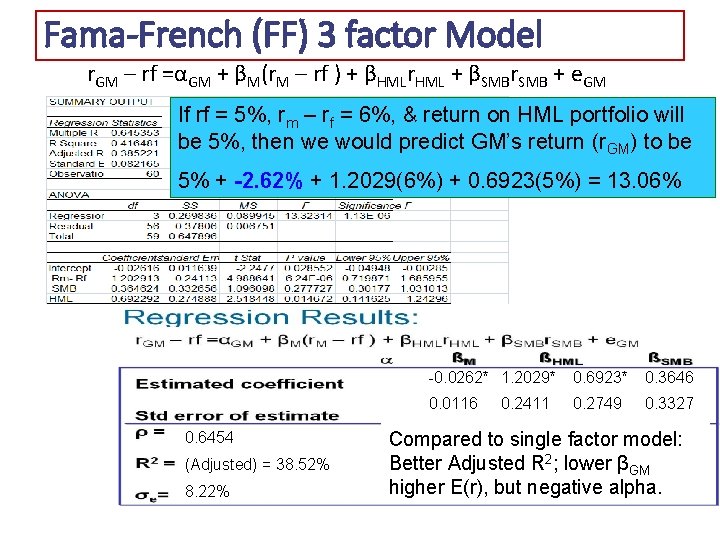
Fama-French (FF) 3 factor Model r. GM – rf =αGM + βM(r. M – rf ) + βHMLr. HML + βSMBr. SMB + e. GM If rf = 5%, rm – rf = 6%, & return on HML portfolio will be 5%, then we would predict GM’s return (r. GM) to be 5% + -2. 62% + 1. 2029(6%) + 0. 6923(5%) = 13. 06% 0. 6454 (Adjusted) = 38. 52% 8. 22% -0. 0262* 1. 2029* 0. 6923* 0. 3646 0. 0116 0. 2749 0. 3327 0. 2411 Compared to single factor model: Better Adjusted R 2; lower βGM higher E(r), but negative alpha.