Lecture 4 Econometric Foundations Stephen P Ryan Olin

Lecture 4: Econometric Foundations Stephen P. Ryan Olin Business School Washington University in St. Louis

Big Question: How to Perform Inference? •

Chernozhukov, Hansen, Spindler (2015)

Basic ideas • Low-dimensional parameter of interest • High-dimensional (infinite? ) nuisance parameter estimated using selection or regularization methods • Provide set of high-level conditions for regular inference • Key condition: immunized or orthogonal estimating equations • Intuition: set up moments so that estimating equations are locally insensitive to small mistakes in nuisance parameters • Application: affine-quadratic models, IV with many regressors and instruments

Setting: High-dimensional models • High-dimensional models, where number of parameters is large relative to sample size, increasingly common/used • Big data -> many covariates • Basis functions -> dictionary of terms for even low-dimensional X • Regularization -> reduction in dimension to focus on “key” components required • Need to account for this regularization when performing inference • General approach -> account for model search (we will talk about this more in moment forests later)

Orthogonality / immunization condition •

Setup •

Adaptivity Condition • We would like to test some hypothesis about the true parameter vector • Inverting test gives us confidence region • Adaptivity is key condition for validity of this inversion: • Key requirement for this to be true is orthogonality / immunization:

Conditions for valid inference • Suppose we have: for some positive-definite • Note that these are at the true values, and are basically telling us the underlying DGP and estimating equations are well-behaved • Suppose there exists a high-quality estimator for the variance:

Then we get something cool • The following score statistic is asymptotically normal: and the quadratic form: • The first equation is what we would like to use in practice!

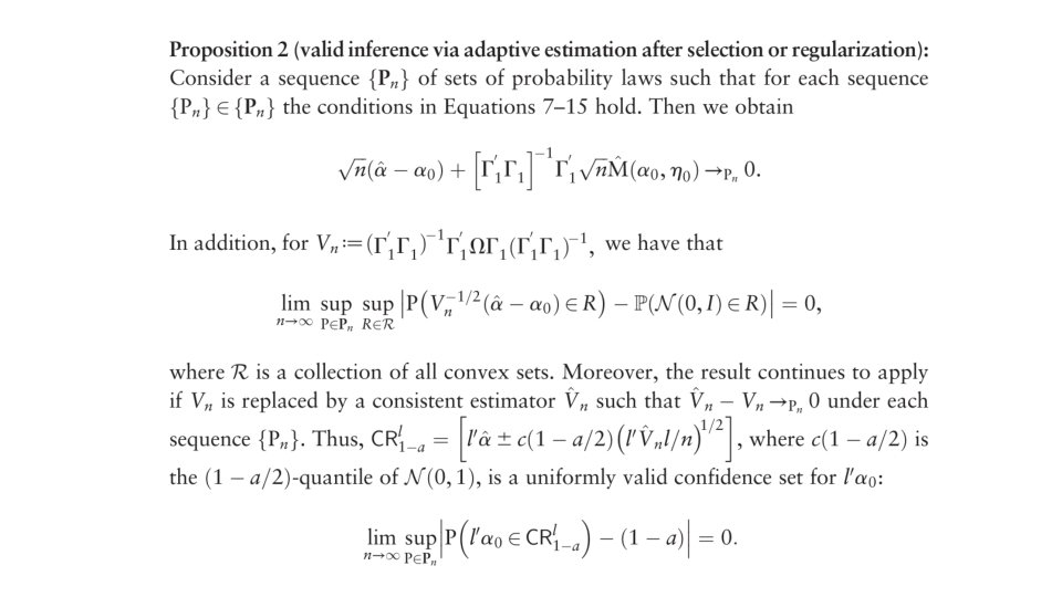
Proposition 1

Valid Inference via Adaptive Estimation •

Achieving Orthogonality • Idea: project score that identifies parameter of interest onto orthocomplement of the tangent space for the nuisance parameter (obviously) • Actually, kind of intuitive partialing out of the nuisance parameter • Suppose we have a likelihood function and: • Consider the following moment function: with:

Orthogonality with Maximum Likelihood • We have both: and

Under true specification • If we assume model is correct, get a nice result: Leading to:

Lemma 1 [Neyman’s Orthogonalization]

Details

Orthogonal GMM Version:

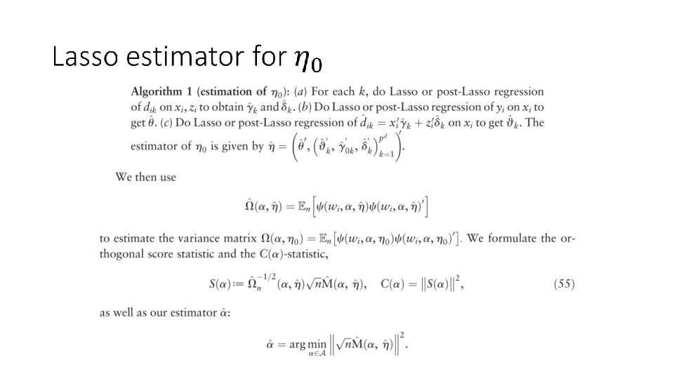
Estimator and Variance

IV with Many Controls and Instruments • Consider a typical IV model, but with many controls (X) and instruments (Z): Where:

IV with Many Controls and Instruments •

Note that we have a bunch of nuisance parameters here •

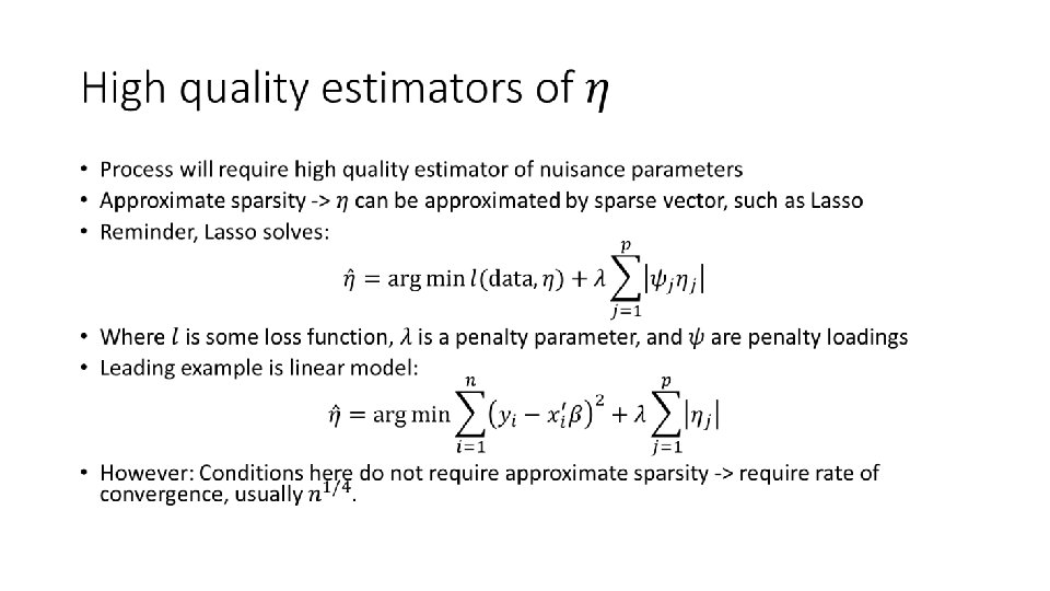
Sparsity •

Condition A 2 + Estimator • Assume that non-sparse component grows at sufficiently slow rate • (by the way, what does that mean in practice? ) • Then, orthogonalized equations are:

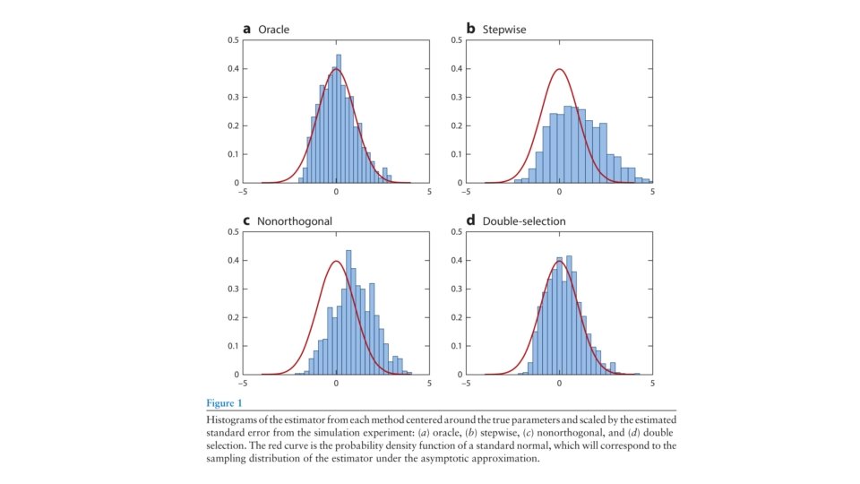
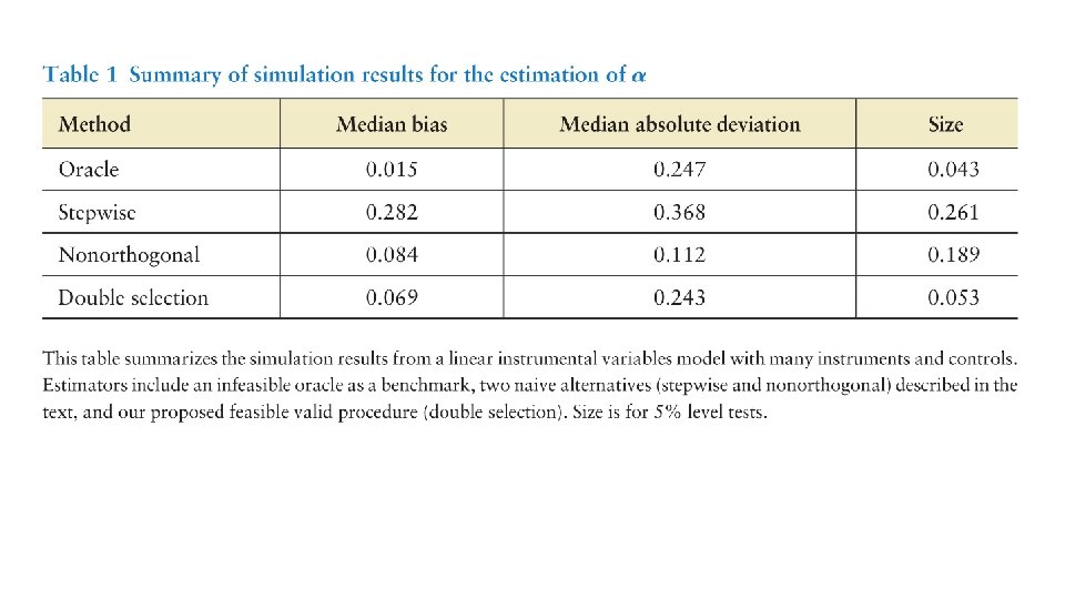
Simulation Results

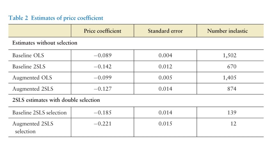
Berry Logit Example ala BLP • Simple aggregate logit model of demand for cars: • Concern: price correlated with unobserved quality • BLP instruments: functions of characteristics of other products • BLP reduced dimensionality to:

This method applied here • In principle, all functions of other product characteristics will be valid instruments • Which ones to use? • CHS propose all first-order interactions of baseline, quadratics, cubics and a time trend • Apply the IV estimator described previously

Conclusion • This paper provides general conditions under which one can perform regular inference after regularizing a high-dimensional set of nuisance parameters • This applies to a very wide set of models • Increasing number of X due to big data • Increasing number of X due to dictionary of basis functions • Two worked examples • Likelihood • GMM • Application to IV • This should be very useful to you all in your own applied work, fairly easy to modify the standard approaches to use