Lecture 12 AO Control Theory Claire Max with

Lecture 12 AO Control Theory Claire Max with many thanks to Don Gavel and Don Wiberg UC Santa Cruz February 18, 2016 Page 1

What are control systems? • Control is the process of making a system variable adhere to a particular value, called the reference value. • A system designed to follow a changing reference is called tracking control or servo. Page 2

Outline of topics • What is control? - The concept of closed loop feedback control • A basic tool: the Laplace transform - Using the Laplace transform to characterize the time and frequency domain behavior of a system - Manipulating Transfer functions to analyze systems • How to predict performance of the controller Page 3

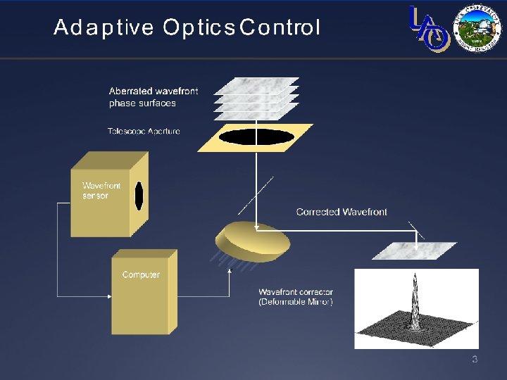
Page 4

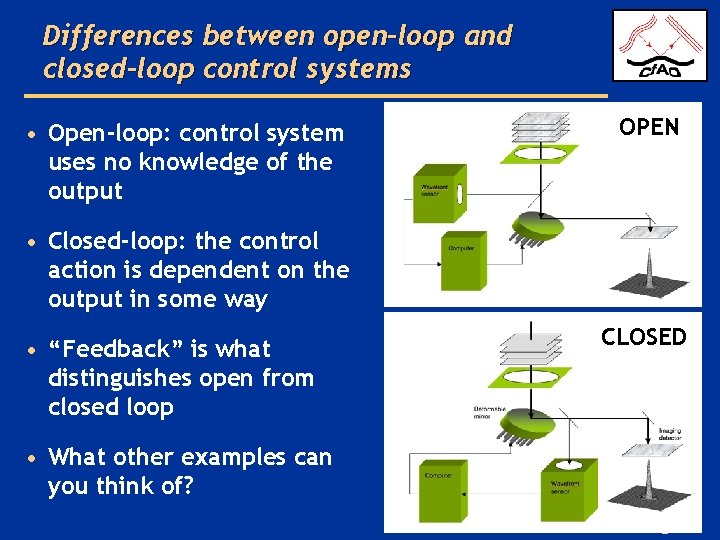
Differences between open-loop and closed-loop control systems • Open-loop: control system uses no knowledge of the output OPEN • Closed-loop: the control action is dependent on the output in some way • “Feedback” is what distinguishes open from closed loop CLOSED • What other examples can you think of? Page 5

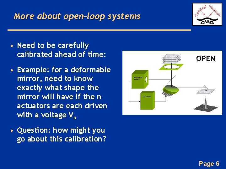
More about open-loop systems • Need to be carefully calibrated ahead of time: OPEN • Example: for a deformable mirror, need to know exactly what shape the mirror will have if the n actuators are each driven with a voltage Vn • Question: how might you go about this calibration? Page 6

Some Characteristics of Closed- Loop Feedback Control • Increased accuracy (gets to the desired final position more accurately because small errors will get corrected on subsequent measurement cycles) • Less sensitivity to nonlinearities (e. g. hysteresis in the deformable mirror) because the system is always making small corrections to get to the right place • Reduced sensitivity to noise in the input signal • BUT: can be unstable under some circumstances (e. g. if gain is too high) Page 7

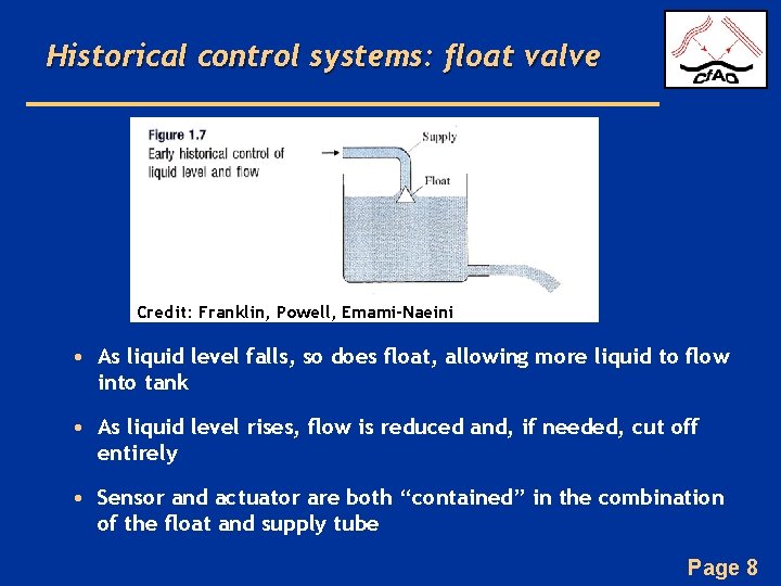
Historical control systems: float valve Credit: Franklin, Powell, Emami-Naeini • As liquid level falls, so does float, allowing more liquid to flow into tank • As liquid level rises, flow is reduced and, if needed, cut off entirely • Sensor and actuator are both “contained” in the combination of the float and supply tube Page 8

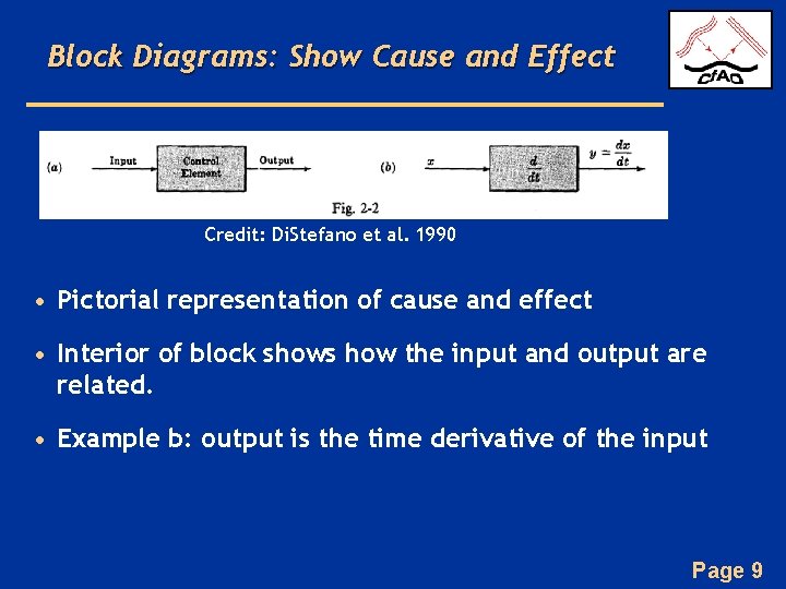
Block Diagrams: Show Cause and Effect Credit: Di. Stefano et al. 1990 • Pictorial representation of cause and effect • Interior of block shows how the input and output are related. • Example b: output is the time derivative of the input Page 9

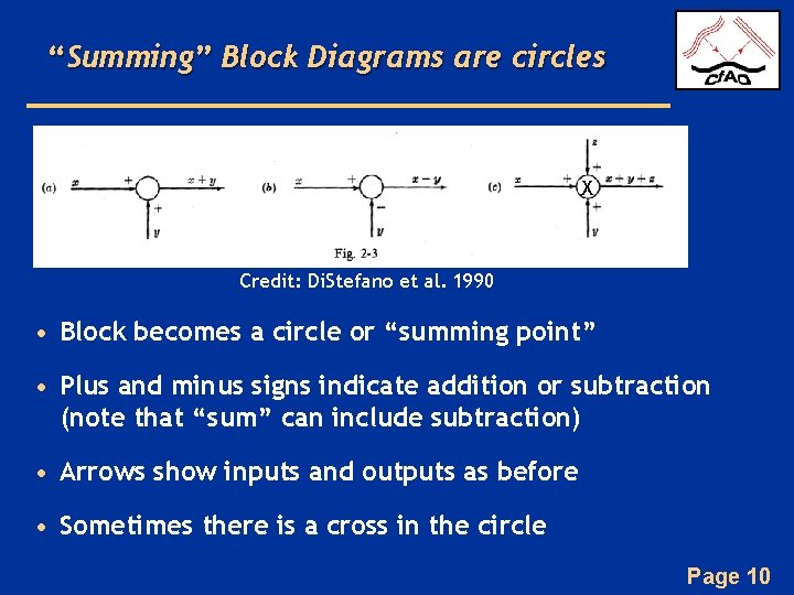
“Summing” Block Diagrams are circles X Credit: Di. Stefano et al. 1990 • Block becomes a circle or “summing point” • Plus and minus signs indicate addition or subtraction (note that “sum” can include subtraction) • Arrows show inputs and outputs as before • Sometimes there is a cross in the circle Page 10

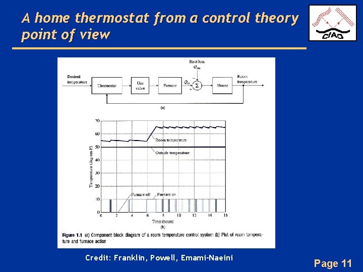
A home thermostat from a control theory point of view Credit: Franklin, Powell, Emami-Naeini Page 11

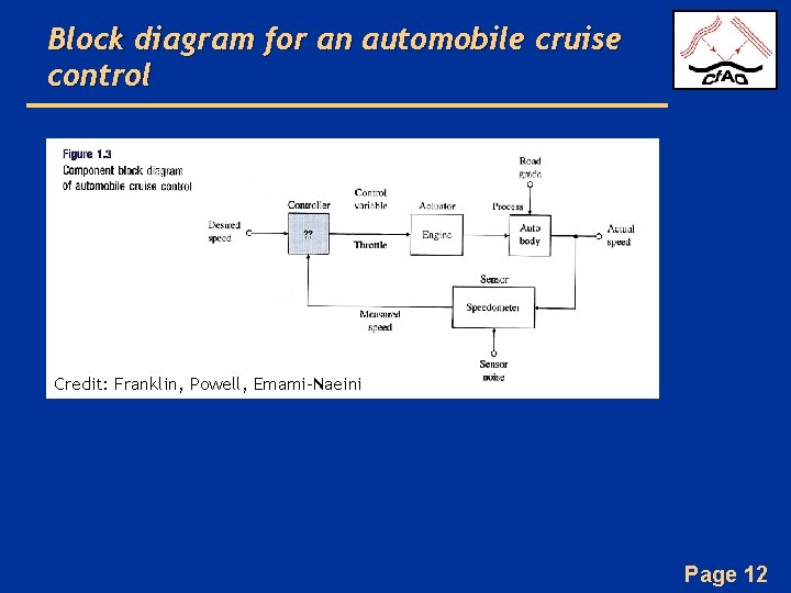
Block diagram for an automobile cruise control Credit: Franklin, Powell, Emami-Naeini Page 12

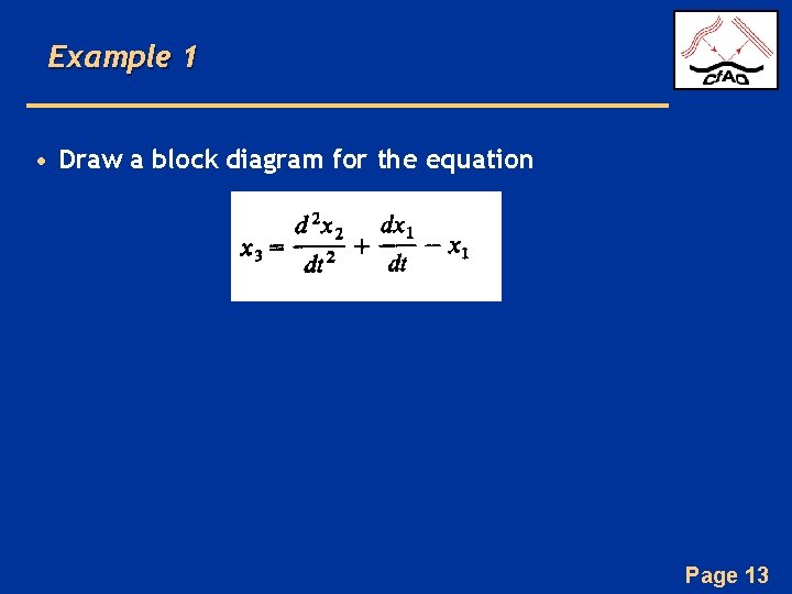
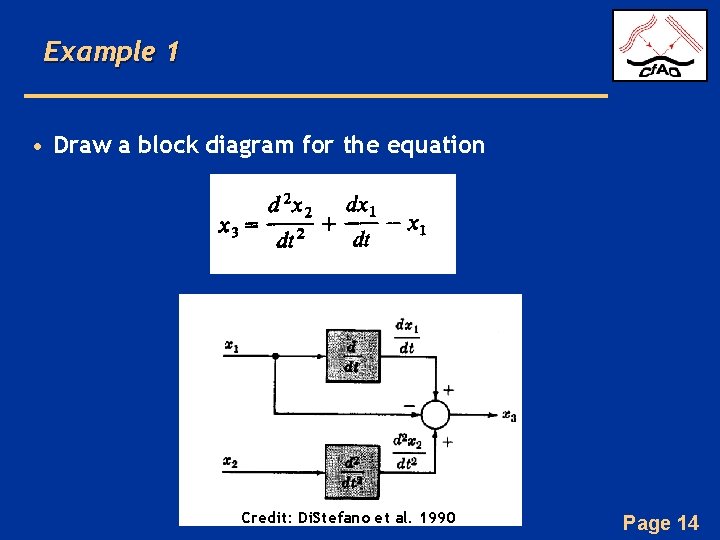
Example 1 • Draw a block diagram for the equation Page 13

Example 1 • Draw a block diagram for the equation Credit: Di. Stefano et al. 1990 Page 14

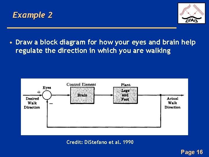
Example 2 • Draw a block diagram for how your eyes and brain help regulate the direction in which you are walking Page 15

Example 2 • Draw a block diagram for how your eyes and brain help regulate the direction in which you are walking Credit: Di. Stefano et al. 1990 Page 16

Summary so far • Distinction between open loop and closed loop – Advantages and disadvantages of each • Block diagrams for control systems – Inputs, outputs, operations – Closed loop vs. open loop block diagrams Page 17

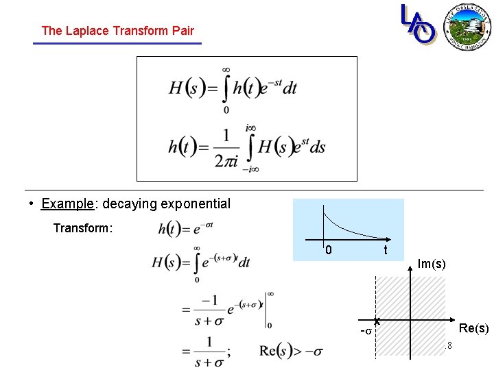
The Laplace Transform Pair • Example: decaying exponential Transform: 0 t Im(s) -σ x Re(s) 18

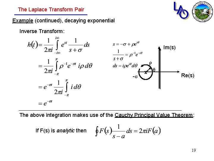
The Laplace Transform Pair Example (continued), decaying exponential Inverse Transform: Im(s) ρ -σ x θ Re(s) The above integration makes use of the Cauchy Principal Value Theorem: If F(s) is analytic then 19

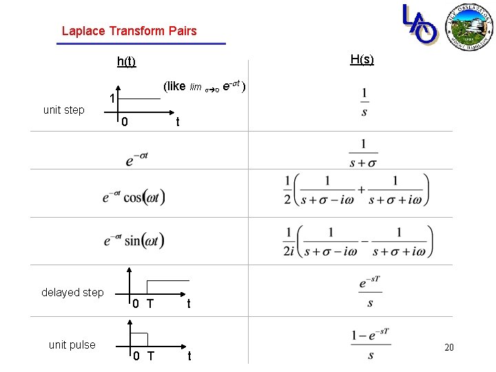
Laplace Transform Pairs H(s) h(t) unit step delayed step unit pulse (like lim s 0 e-st ) 1 0 t 0 T t 20

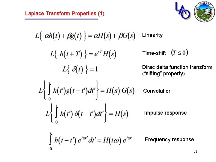
Laplace Transform Properties (1) Linearity Time-shift Dirac delta function transform (“sifting” property) Convolution Impulse response Frequency response 21

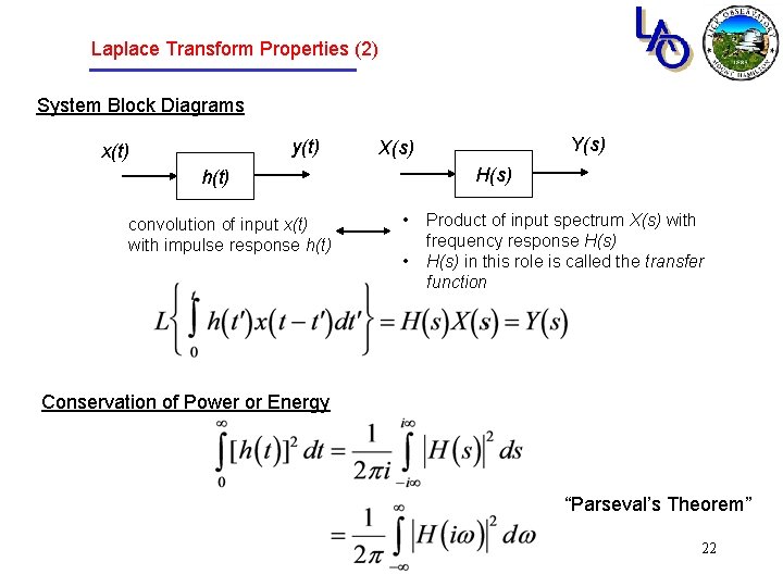
Laplace Transform Properties (2) System Block Diagrams y(t) x(t) H(s) h(t) convolution of input x(t) with impulse response h(t) Y(s) X(s) • • Product of input spectrum X(s) with frequency response H(s) in this role is called the transfer function Conservation of Power or Energy “Parseval’s Theorem” 22

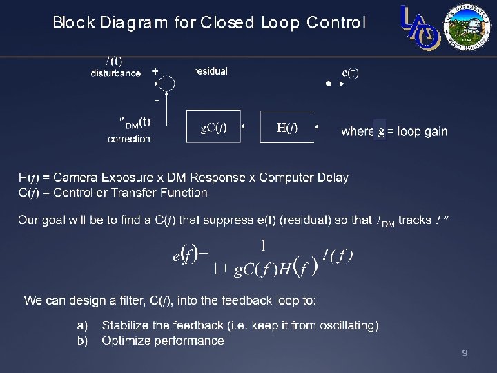
Closed loop control (simple example, H(s)=1) W(s) disturbance X(s) + - E(s) residual Y(s) correction g. C(s) Where gain Our goal will be to suppress X(s) (residual) by high-gain feedback so that Y(s)~W(s) solving for E(s), Note: for consistency “around the loop, ” the units of the gain g must be the inverse of the units of C(s). 23

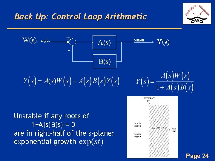
Back Up: Control Loop Arithmetic W(s) input + - A(s) output Y(s) B(s) Unstable if any roots of 1+A(s)B(s) = 0 are in right-half of the s-plane: exponential growth Page 24

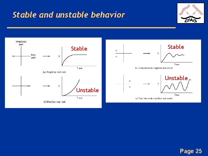
Stable and unstable behavior Stable Unstable Page 25

g Page 26

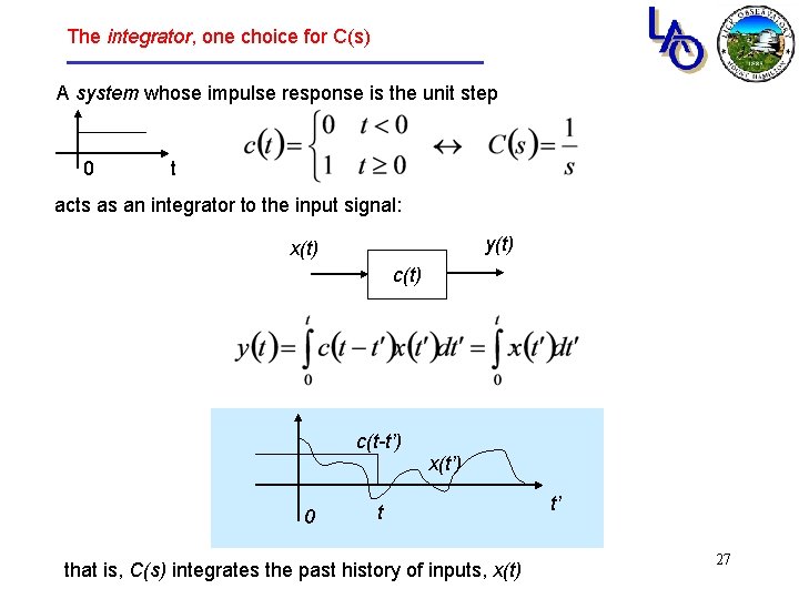
The integrator, one choice for C(s) A system whose impulse response is the unit step 0 t acts as an integrator to the input signal: y(t) x(t) c(t-t’) x(t’) 0 t that is, C(s) integrates the past history of inputs, x(t) t’ 27

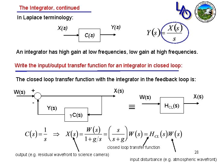
The Integrator, continued In Laplace terminology: Y(s) X(s) C(s) An integrator has high gain at low frequencies, low gain at high frequencies. Write the input/output transfer function for an integrator in closed loop: The closed loop transfer function with the integrator in the feedback loop is: W(s) + - X(s) W(s) HCL(s) Y(s) g. C(s) closed loop transfer function output (e. g. residual wavefront to science camera) 28 input disturbance (e. g. atmospheric wavefront)

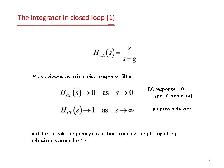
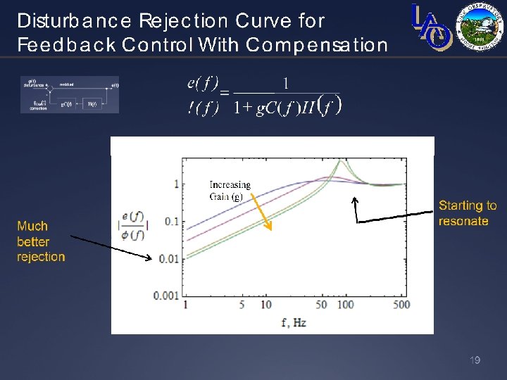
The integrator in closed loop (1) HCL(s), viewed as a sinusoidal response filter: DC response = 0 (“Type-0” behavior) High-pass behavior and the “break” frequency (transition from low freq to high freq behavior) is around s ~ g 29

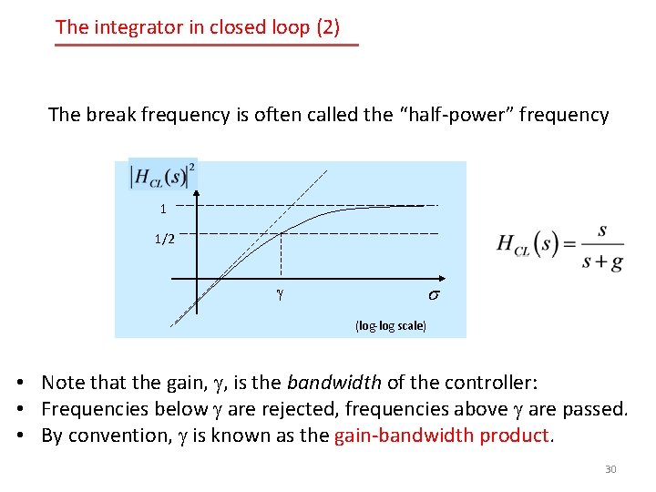
The integrator in closed loop (2) The break frequency is often called the “half-power” frequency 1 1/2 g s (log-log scale) • Note that the gain, g, is the bandwidth of the controller: • Frequencies below g are rejected, frequencies above g are passed. • By convention, g is known as the gain-bandwidth product. 30

Page 31

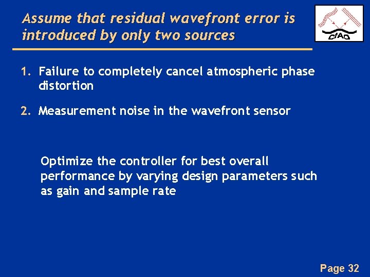
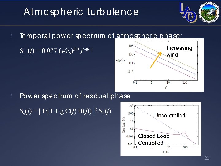
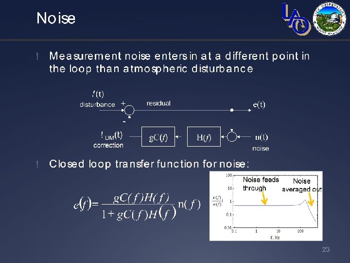
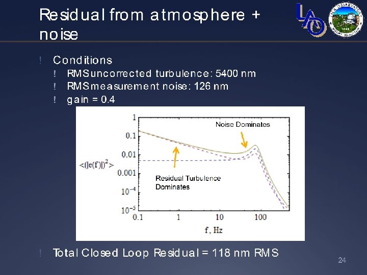
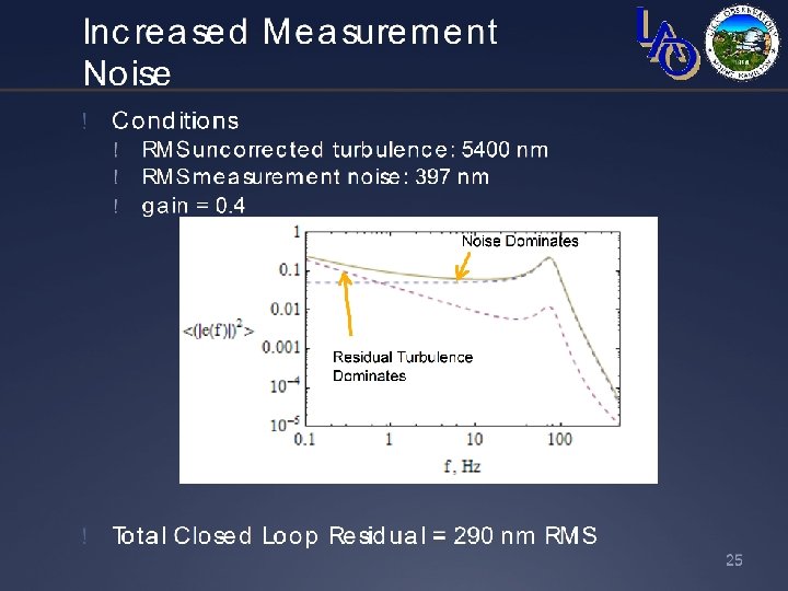
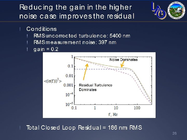
Assume that residual wavefront error is introduced by only two sources 1. Failure to completely cancel atmospheric phase distortion 2. Measurement noise in the wavefront sensor Optimize the controller for best overall performance by varying design parameters such as gain and sample rate Page 32

Page 33

Page 34

Page 35

Page 36

Page 37

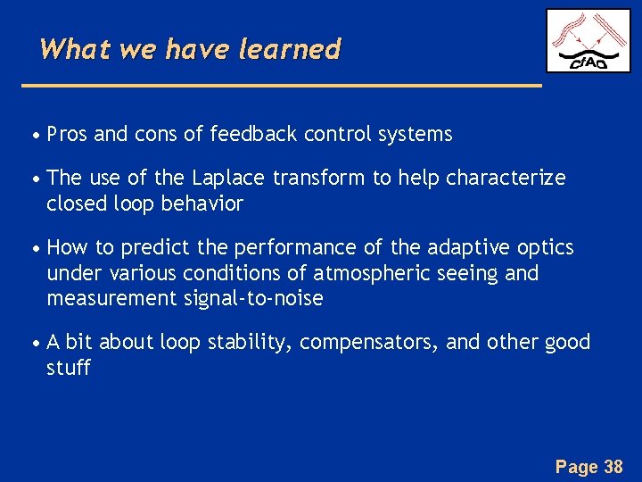
What we have learned • Pros and cons of feedback control systems • The use of the Laplace transform to help characterize closed loop behavior • How to predict the performance of the adaptive optics under various conditions of atmospheric seeing and measurement signal-to-noise • A bit about loop stability, compensators, and other good stuff Page 38

Page 39