Last Time Scattering theory Integrating tranfer equations 022805

Last Time • Scattering theory • Integrating tranfer equations 02/28/05 © 2005 University of Wisconsin

Today • Sub-surface scattering • Sky models 02/28/05 © 2005 University of Wisconsin

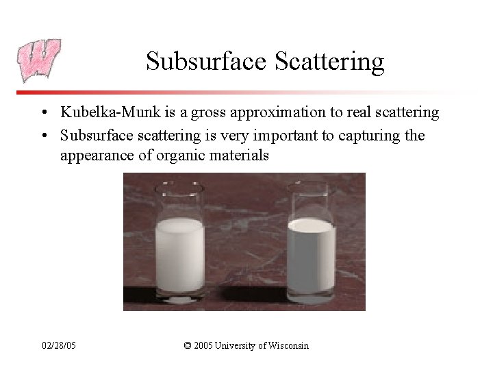
Subsurface Scattering • Kubelka-Munk is a gross approximation to real scattering • Subsurface scattering is very important to capturing the appearance of organic materials 02/28/05 © 2005 University of Wisconsin

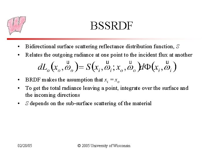
BSSRDF • Bidirectional surface scattering reflectance distribution function, S • Relates the outgoing radiance at one point to the incident flux at another • BRDF makes the assumption that xi = xo • To get the total radiance leaving a point, integrate over the surface and the incoming directions • S depends on the sub-surface scattering of the material 02/28/05 © 2005 University of Wisconsin

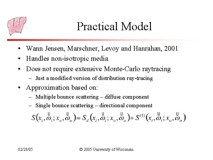
Practical Model • Wann Jensen, Marschner, Levoy and Hanrahan, 2001 • Handles non-isotropic media • Does not require extensive Monte-Carlo raytracing – Just a modified version of distribution ray-tracing • Approximation based on: – Multiple bounce scattering – diffuse component – Single bounce scattering – directional component 02/28/05 © 2005 University of Wisconsin

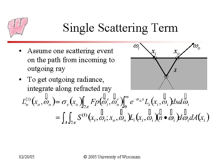
Single Scattering Term • Assume one scattering event on the path from incoming to outgoing ray • To get outgoing radiance, integrate along refracted ray 02/28/05 i © 2005 University of Wisconsin xi xo s o

Single Scattering Term • S(1) is defined by this formula 02/28/05 © 2005 University of Wisconsin

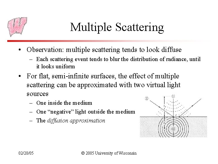
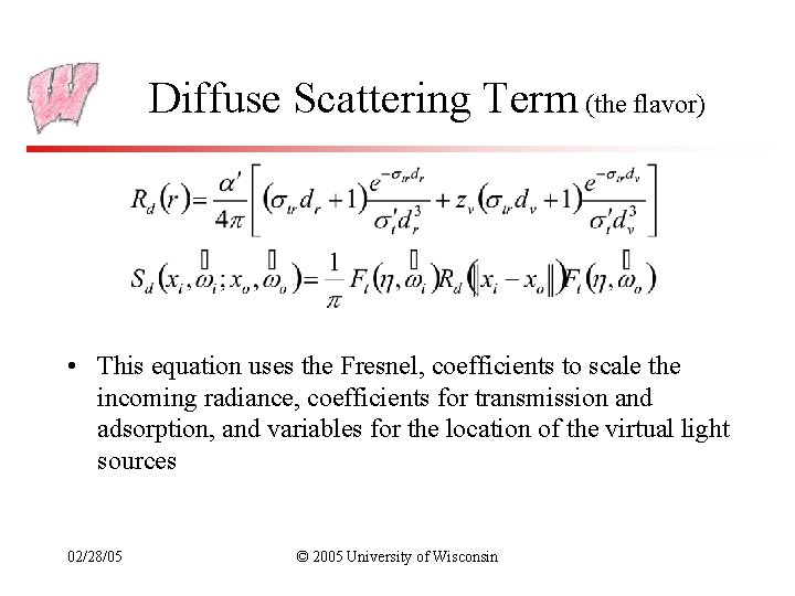
Multiple Scattering • Observation: multiple scattering tends to look diffuse – Each scattering event tends to blur the distribution of radiance, until it looks uniform • For flat, semi-infinite surfaces, the effect of multiple scattering can be approximated with two virtual light sources – One inside the medium – One “negative” light outside the medium – The diffusion approximation 02/28/05 © 2005 University of Wisconsin

Diffuse Scattering Term (the flavor) • This equation uses the Fresnel, coefficients to scale the incoming radiance, coefficients for transmission and adsorption, and variables for the location of the virtual light sources 02/28/05 © 2005 University of Wisconsin

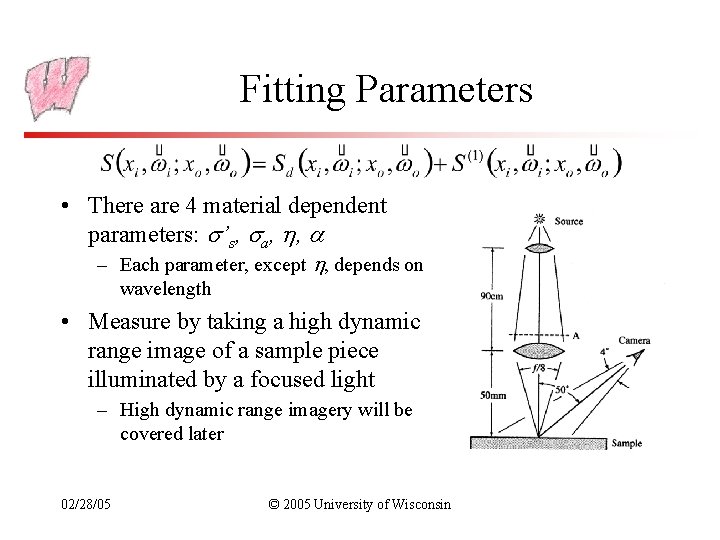
Fitting Parameters • There are 4 material dependent parameters: ’s, a, , – Each parameter, except , depends on wavelength • Measure by taking a high dynamic range image of a sample piece illuminated by a focused light – High dynamic range imagery will be covered later 02/28/05 © 2005 University of Wisconsin

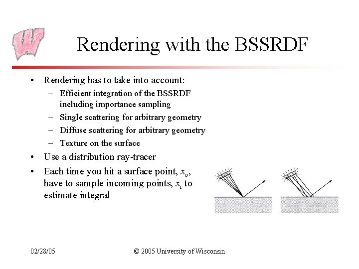
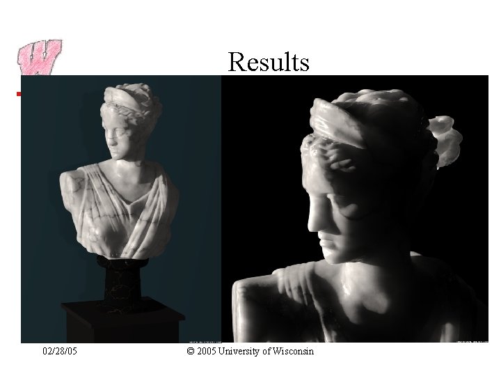
Rendering with the BSSRDF • Rendering has to take into account: – Efficient integration of the BSSRDF including importance sampling – Single scattering for arbitrary geometry – Diffuse scattering for arbitrary geometry – Texture on the surface • Use a distribution ray-tracer • Each time you hit a surface point, xo, have to sample incoming points, xi to estimate integral 02/28/05 © 2005 University of Wisconsin

Sampling Approaches • For single scattering terms, sample points along the refracted outgoing ray – Cast shadow ray to light to find out incoming radiance – Push this through single scattering equation to get outgoing – Make distant light approximation to ease computations • For diffuse scattering term, sample points around the outgoing point – Then place the virtual lights and evaluate the equation – Must be careful to put virtual lights in appropriate places • For texture, use parameters from xi for diffuse, and combination of xi and xo for single scattering 02/28/05 © 2005 University of Wisconsin

Results 02/28/05 © 2005 University of Wisconsin

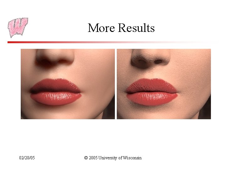
More Results 02/28/05 © 2005 University of Wisconsin

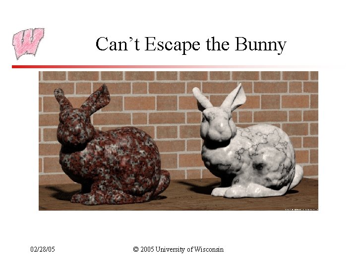
Can’t Escape the Bunny 02/28/05 © 2005 University of Wisconsin

Sky Illumination • The sky is obviously an important source of illumination • The atmosphere is an important participating medium over large distances (hundreds of meters) – People use atmospheric effects to judge distances (stereo and disparity effects are useless at large distances) • Three models: – CIE model – Perez model – Preetham, Shirley and Smits model 02/28/05 © 2005 University of Wisconsin

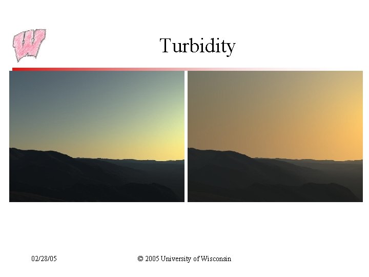
Atmospheric Phenomena • Due to solar illumination and scattering in the atmosphere • Air molecules are modeled by Rayleigh scattering – Optical extinction coefficient varies with -4 – What phenomena does this explain? • Scattering due to larger particles is modeled with Mie scattering – Scattering depends less on wavelength, so what color is haze? • Turbidity is a useful measurement: T=(tm+th)/tm – tm is vertical optical thickness of molecular atmosphere – th is vertical optical thickness of haze atmosphere 02/28/05 © 2005 University of Wisconsin

Simulation Models • These attempt to simulate the scattering in the atmosphere to produce images – Very expensive for practical use – But work with any atmospheric conditions 02/28/05 © 2005 University of Wisconsin

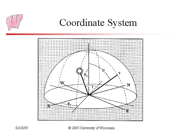
Coordinate System 02/28/05 © 2005 University of Wisconsin

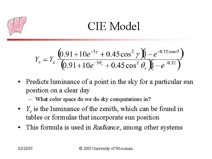
CIE Model • Predicts luminance of a point in the sky for a particular sun position on a clear day – What color space do we do sky computations in? • Yz is the luminance of the zenith, which can be found in tables or formulas that incorporate sun position • This formula is used in Radiance, among other systems 02/28/05 © 2005 University of Wisconsin

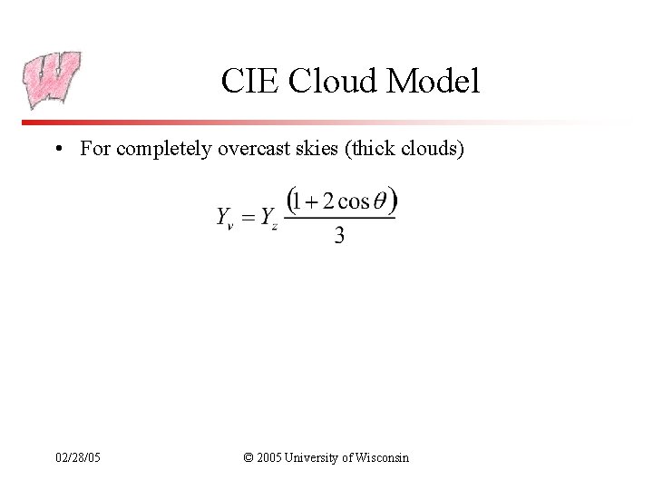
CIE Cloud Model • For completely overcast skies (thick clouds) 02/28/05 © 2005 University of Wisconsin

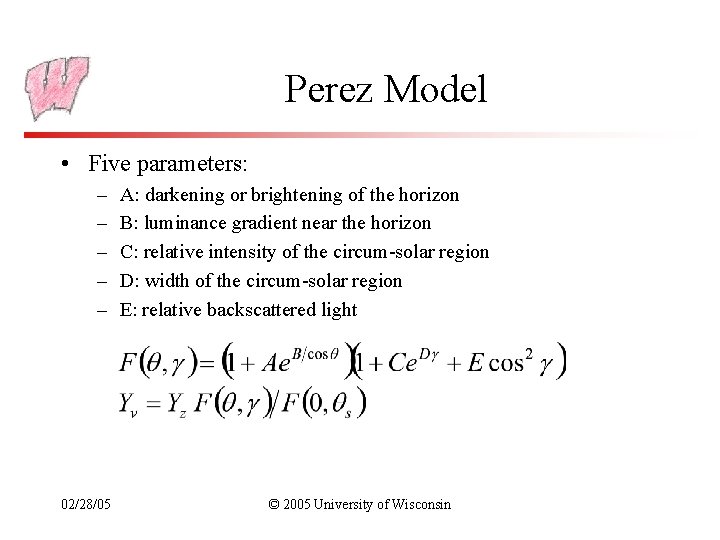
Perez Model • Five parameters: – – – 02/28/05 A: darkening or brightening of the horizon B: luminance gradient near the horizon C: relative intensity of the circum-solar region D: width of the circum-solar region E: relative backscattered light © 2005 University of Wisconsin

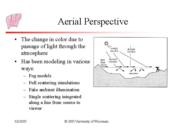
Aerial Perspective • The change in color due to passage of light through the atmosphere • Has been modeling in various ways: – – 02/28/05 Fog models Full scattering simulations Fake ambient illumination Single scattering integrated along a line from source to viewer © 2005 University of Wisconsin

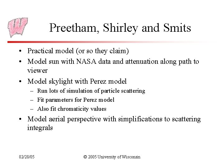
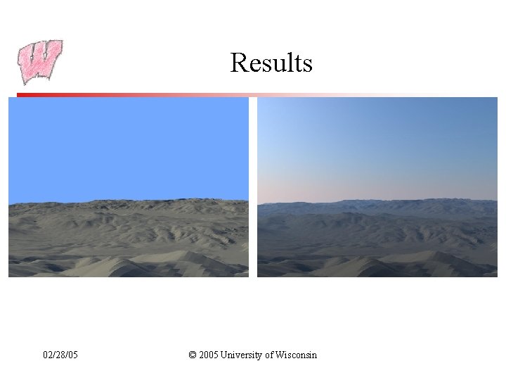
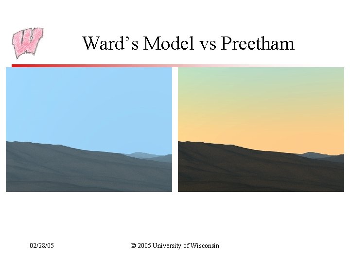
Preetham, Shirley and Smits • Practical model (or so they claim) • Model sun with NASA data and attenuation along path to viewer • Model skylight with Perez model – Run lots of simulation of particle scattering – Fit parameters for Perez model – Also fit chromaticity values • Model aerial perspective with simplifications to scattering integrals 02/28/05 © 2005 University of Wisconsin

Results 02/28/05 © 2005 University of Wisconsin

Turbidity 02/28/05 © 2005 University of Wisconsin

Ward’s Model vs Preetham 02/28/05 © 2005 University of Wisconsin

Next Time • High Dynamic Range 02/28/05 © 2005 University of Wisconsin