Key Issues in Solidification Modeling Vaughan Voller University

Key Issues in Solidification Modeling— Vaughan Voller, University of Minnesota, Aditya Birla Chair Scales: Validation and Verification: Process Micro-strcture ~10 mm Do governing equations model the correct physics? Is approximate solution a solution of governing Equations ? Ferreira et al ~0. 5 m How can we deal with this problem Micro-macro models Prediction Of microstructure How feasible is Direct Modeling of Microstructure? What can it tell us about the process Scale?

Scales: An Example Problem: Macrosegregation—Ingot alloy solidification In mushy region solute is partitioned at solid-liquid interface Result after full solidification is macro-scale areas with concentration above or Below the nominal concentration see Cliquid Csolid Flemings (Solidification Processing) solid crystals + liquid and Beckermann (Ency. Mat) “mushy region” This solute is redistributed at process scale by fluid and solid motions shrinkage solid grain motion convection liquid alloy 1 m

Key Scales in Macro-segregation Process REV representative ½ arm space g solid ~ 50 mm ~0. 5 m Solute transport controlled by advection ~5 mm Computational grid size sub-grid model Solute value in liquid phase controlled by local diffusion in solid “microsegregation”

A Casting chi ll ~ 0. 1 m Scales in General Solidification Processes The REV ~10 mm Nucleation Sites columnar (after Dantzig) 101 The Secondary Arm Space Time Scale (s) ~ mm grain formation 10 -1 growth 10 -3 10 -5 solute diffusion nucleation 10 -7 interface kinetics 10 -9 The Tip Radius ~10 mm ~1 nm f= 1 f = -1 heat and mass tran. equi-axed The Grain Envelope ~100 mm casting 103 The Diffusive Interface 10 10 -3 Length Scale (m) 10 -1 Question for later: Can we build a direct-simulation of a Casting Process that resolves to all scales?

A solidification model has three components: The Domain: The Grid: The sub-Grid: Examples Problem Domains Macro Process The Grid Realizations--Of multi-phase regions Element in numerical Calculation ---REV State described by averaged mixture values REV Sub-grid --Constitutive -Controlled by averaged Properties in REV Effect of morphology on flow METER Meso Microstructure The Grain Envelope Solid-liquid interface A representative Arm spacing— Form of Constitutive model T=F(g) f= 1 f = -1 The Diffusive Interface, e. g. NANO-Meter

Key Scales in Macro-segregation Process REV representative ½ arm space g solid ~ 50 mm ~5 mm ~0. 5 m Computational grid size Solute transport controlled by advection sub-grid model Solute value in liquid phase controlled by local diffusion in solid “microsegregation” Develop a “Macro-Micro Model” (Rappaz) Solve transport equations at macroscopic scale (MACRO) Use sub-grid model to account for microsegregation (MICRO) a “constitutive model”

Macro (Process) Scale Equations of Motion (Flows) REV mm Heat: Solute Concentrations: Assumptions for shown Eq. s: -- No solid motion --U is inter-dendritic volume flow If a time explicit scheme is used to advance to the next time step we need find REV values for • T temperature • Cl liquid concentration • gs solid fraction • Cs(x) distribution of solid concentration

The Micro-Macro Model MACRO: Process REV MICRO: representative ½ arm space g solid sub-grid model ~0. 5 m ~5 mm ~ 50 mm microsegregation and solute diffusion in arm space Computational grid size from computation Of these Mixture values need to extract -- -- --

Primary Solidification Solver g Transient mass balance g model of micro-segregation T Iterative loop (will need under-relaxation) Cl Gives Liquid Concentrations A C equilibrium

Micro-segregation Model liquid concentration due to macro-segregation alone ½ Arm space of length l takes tf seconds to solidify In a small time step new solid forms with lever rule of concentration transient mass balance gives liquid concentration Solute Fourier No. Solute mass density before solidification Solute mass density after solidification Solute mass density of new solid (lever) Q -– back-diffusion Need an easy to use approximation For back-diffusion

The parameter Model --- Clyne and Kurz, For special case Of Parabolic Solid Growth and Ohnaka In Most other cases The Ohnaka approximation And ad-hoc fit sets the factor Works very well

The Profile Model Wang and Beckermann Need to lag calculation one time step and ensure Q >0 m is sometimes take as a constant ~ 2 BUT In the time step model a variable value can be use Due to steeper profile at low liquid fraction ----- Propose

An Important wrinkle ---Coarsening Due to dissolution processes some arms will melt and arm-space will coarsen Time 1 Time 2 > Time 1

Coarsening Arm-space will increase in dimension with time This will dilute the concentration in the liquid fraction—can model be enhancing the back diffusion A model by Voller and Beckermann suggests If we assume that solid growth is close to parabolic m =2. 33 in Parameter model In profile model

Verification: of Micro Models: Constant Cooling of Binary-Eutectic Alloy With Initial Concentration C 0 = 1 and Eutectic Concentration Ceut = 5, No Macro segregation , k = 0. 1 T Cl As solidification proceeds the concentration in liquid increases. When the eutectic composition is reached remaining liquid solidifies isothermally, Eutectic Fraction In model calculate the transient value of g from Use 200 time steps and equally increment 1 < Cl < 5 Parameter or Profile

Verification of Micro Models: Verify approximate model for back-diffusion by comparing solution with FD solution of Fick’s equation in arm space. Parameter or Profile Remaining Liquid when C =5 is Eutectic Fraction

Validation of Micro Model: Predictions of Eutectic Fraction With constant cooling Co = 4. 9 Ceut = 33. 2 k = 0. 16 Al-4. 9% Cu Comparison with Experiments Sarreal-Abbaschian Met Trans 1986 X-ray analysis determines average eutectic fraction

Macro-Micro Model of Solidification Calculate predict T Predict g Transient solute balance in arm space A predict Cl C My Method of Choice Parameter Two MICRO Models For Back Diffusion Profile Robust Easy to Use Poor Performance at very low liquid fraction— can be corrected A little more difficult to use Account for coarsening With this Ad-hoc correction Excellent performance at all ranges

Modeling the fluid flow could require a Two Phase model, that may need to account for: Both Solid and Liquid Velocities at low solid fractions A switch-off of the solid velocity in a columnar region A switch-off of velocity as solid fraction g o. An EXAMPLE 2 -D form of the momentum equations in terms of the interdentrtic fluid flow U, are: Extra Terms Magically vanish Buoyancy Friction between solid and liquid Accounts for mushy region morphology Can requires a solid-momentum equation

Verification: of Macro-Micro Model—Inverse Segregation in a Binary Alloy riser liquid 100 mm Shrinkage sucks solute rich fluid toward chill – results in a region of +ve segregation at chill mushy y solid chill Fixed temp chill results in a similarity solution Flow by simple app. of continuity Parameter Current estimate empirical

Validation: Comparison with Experiments riser liquid 100 mm mushy y solid chill Ferreira et al Met Trans 2004

Direct Microstructure Modeling A Casting chi ll ~ 0. 1 m domain The REV ~10 mm Nucleation Sites columnar grid equi-axed domain The Grain Envelope ~ mm The Secondary Arm Space ~100 mm The Tip Radius ~10 mm ~1 nm f= 1 f = -1 sub-grid Macro-Micro models at process scale The Diffusive Interface constitutive grid Micro-Nano model for micro-structure

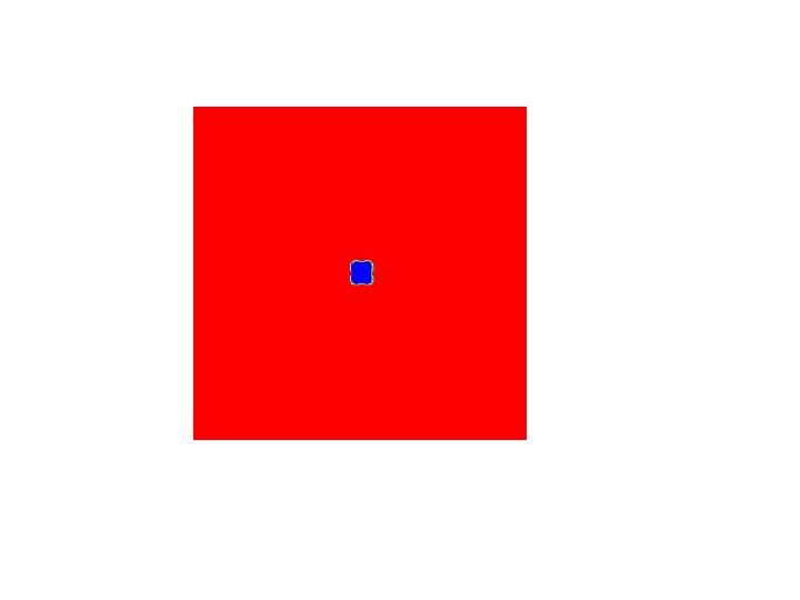
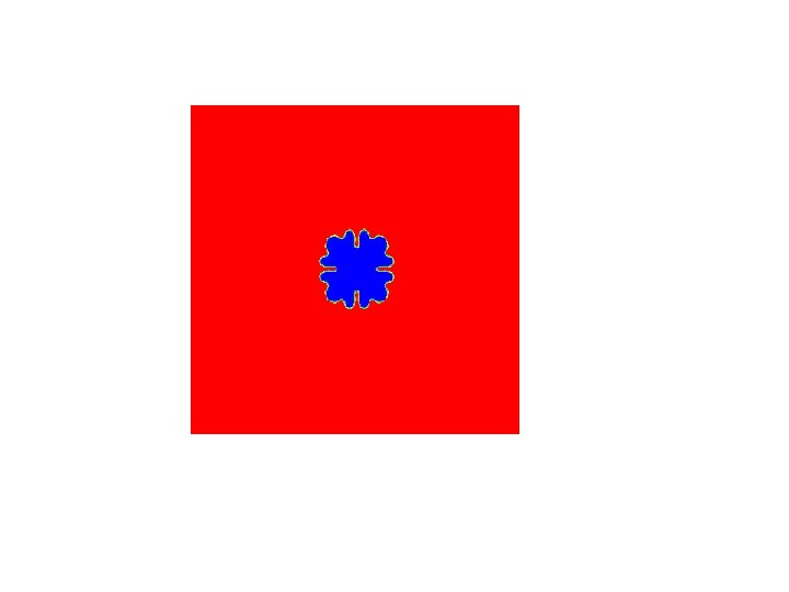
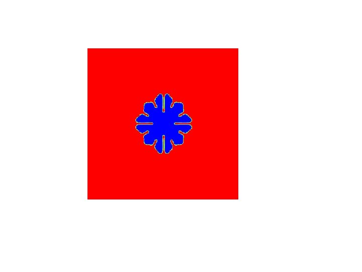
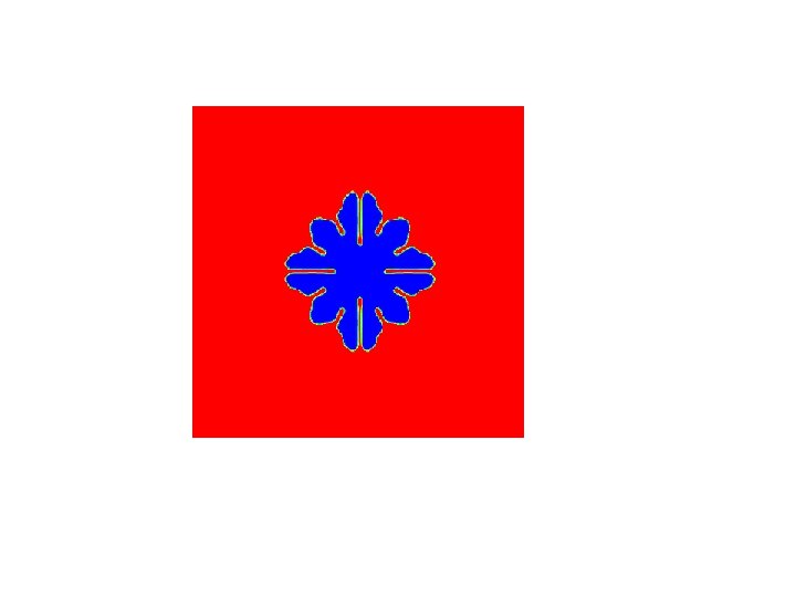
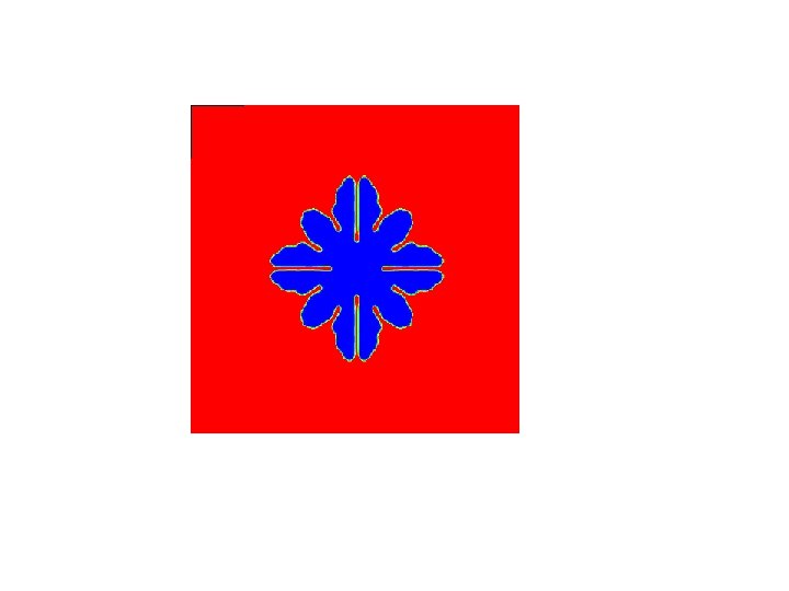
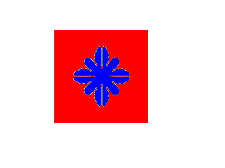
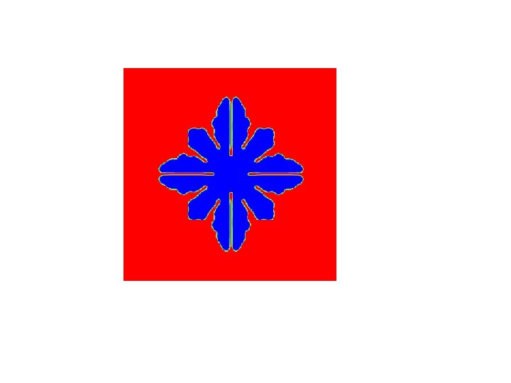
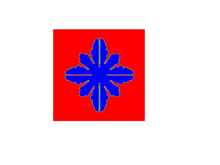
Example: Growth of dendritic crystal in an under-cooled melt (seminar on July 14) Solved in ¼ Domain with A 200 x 200 grid Growth of solid seed in a liquid melt Initial dimensionless undercooling T = -0. 8 Resulting crystal has an 8 fold symmetry

Grid independent results with correct dynamics can be readily obtained Tip Velocity grid anisotropy Interacting grains prediction of concentration field Scale of calculations shown 1 mm

So can we use DMS to predict microstructure at the process level? Process ~0. 5 m REV ~5 mm ~ 1 mm Computational grid size Sub grid scale For 2 -D calc at this scale Will need 1018 grids

For 2 -D calc at this scale Will need 1018 grids Voller and Porte-Agel, JCP 179, 698 -703 (2002 1000 20. 6667 Year “Moore’s Law” 2055

CONCLUSIONS A Casting chi ll ~ 0. 1 m The REV ~10 mm Nucleation Sites columnar equi-axed The Grain Envelope ~ mm Validated and Verified Models that Can successfully model across ~ 4 decades Of length scales Able to use Macro-Micro Approach To model all scales of Heat and Mass Transport Able to build Local Microstructure models The Secondary Arm Space ~100 mm But a long way from DMS Direct microstructure simulation at the process scale The Tip Radius ~10 mm ~1 nm Conclusion: Can Currently Build f= 1 f = -1 The Diffusive Interface In the meantime what Value Added can we get from Local microstructure models Use as generator for constitutive models Use in volume averaging approaches