JPMTAnalogue Signal Processor PMT analogue signal processor in

JPMTAnalogue. Signal. Processor PMT analogue signal processor in Jpp M. de Jong 1

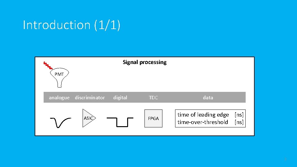
Introduction (1/1) Signal processing PMT analogue discriminator ASIC digital TDC FPGA data time of leading edge [ns] time-over-threshold [ns] 2

Introduction (2/3) amplitude [p. e. ] definition gain spread threshold time-over-threshold time 3

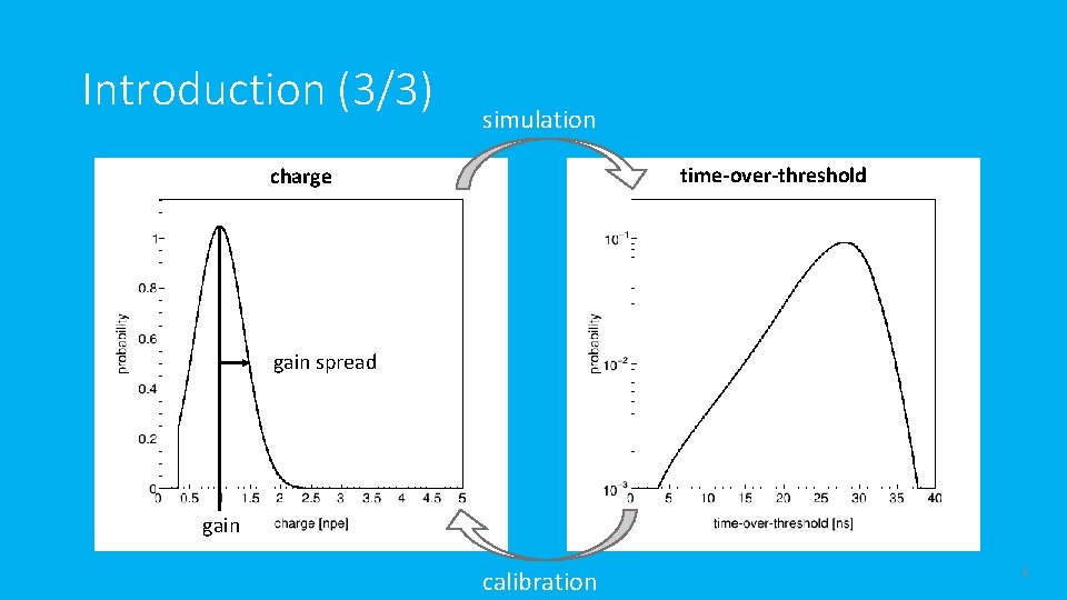
Introduction (3/3) simulation time-over-threshold charge gain spread gain calibration 4

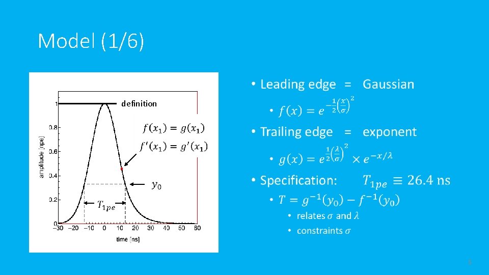
Model (1/6) • definition 5

Model (2/6) 2 number of hits [a. u. ] Bram Schermer 1 (Nikhef) 3 4 5 peak 1 2 3 ns 27 35 42 4 5 6 49 56 62 6 time over threshold [ns] 6

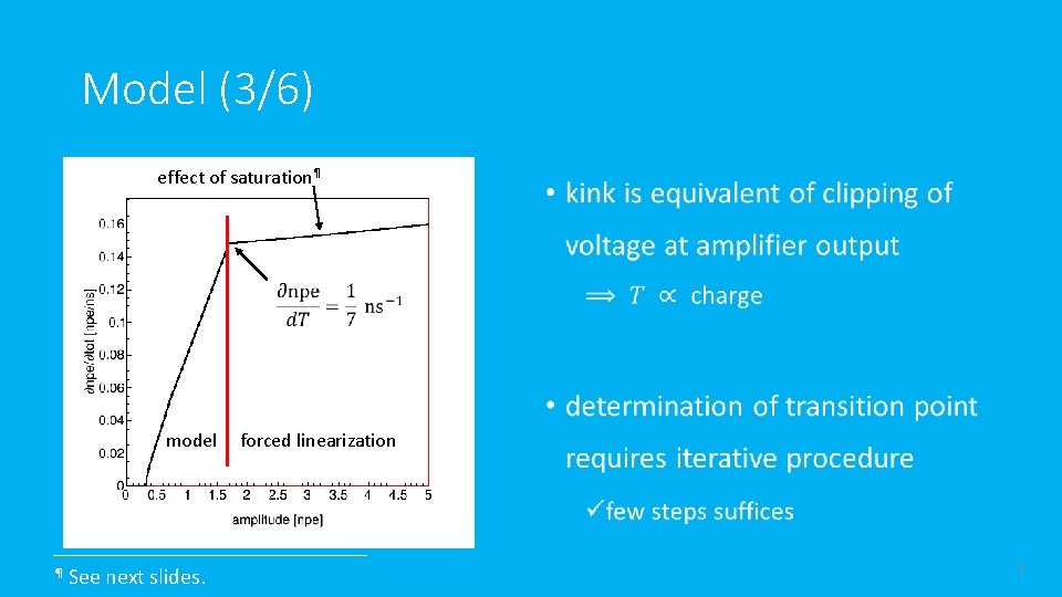
Model (3/6) effect of saturation¶ model ¶ See next slides. • forced linearization 7

Model (4/6) number of hits [a. u. ] Model for given number of photo-electrons time over threshold [ns] 8

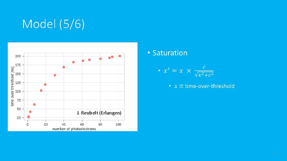
Model (5/6) • J. Reubelt (Erlangen) 9

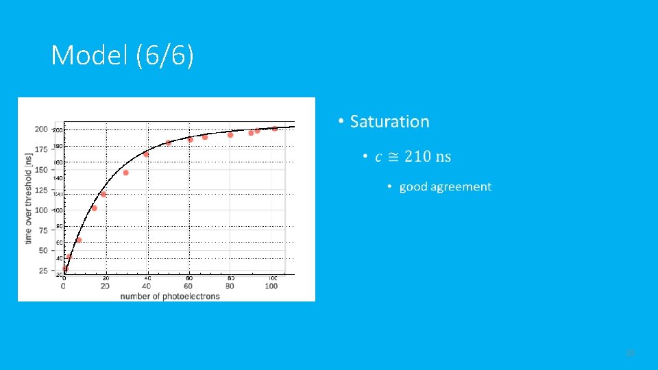
Model (6/6) • 10

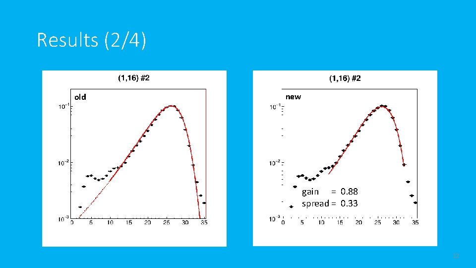
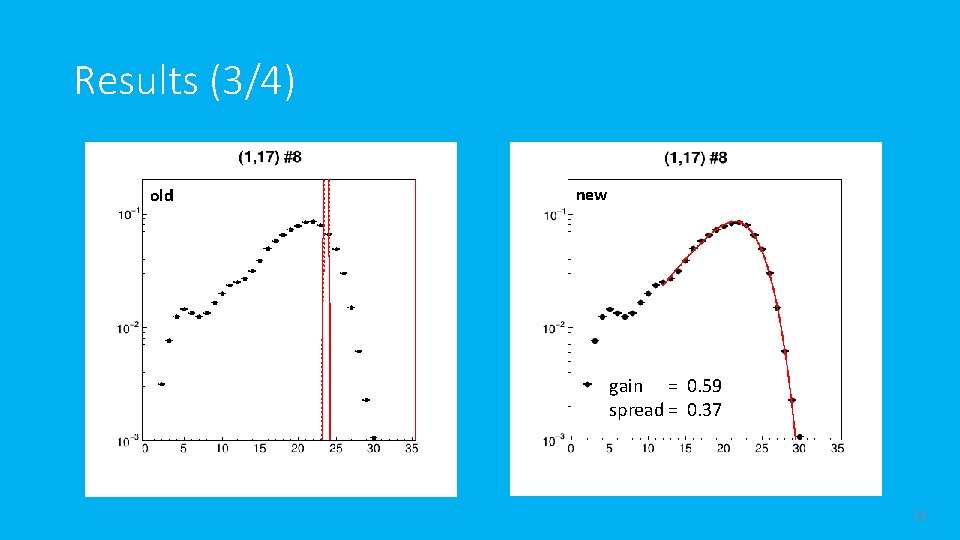
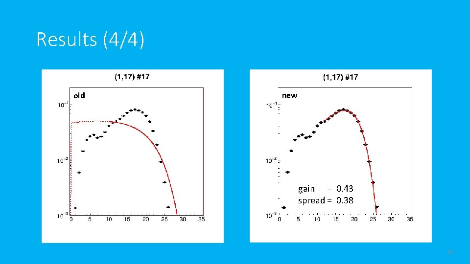
Results (1/4) • input KM 3 Ne. T_00000014_00005282. root (L 0 data) • old = Jpp trunk (11531) • new = this analysis 11

Results (2/4) old new gain = 0. 88 spread = 0. 33 12

Results (3/4) old new gain = 0. 59 spread = 0. 37 13

Results (4/4) old new gain = 0. 43 spread = 0. 38 14

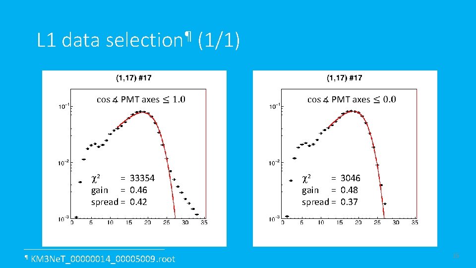
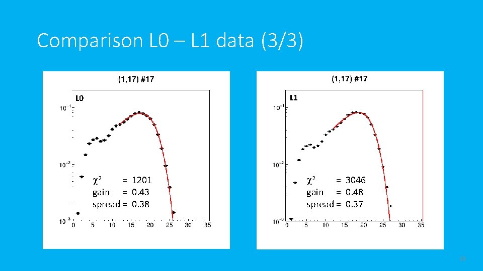
L 1 data selection¶ (1/1) c 2 = 33354 gain = 0. 46 spread = 0. 42 ¶ KM 3 Ne. T_00000014_00005009. root c 2 = 3046 gain = 0. 48 spread = 0. 37 15

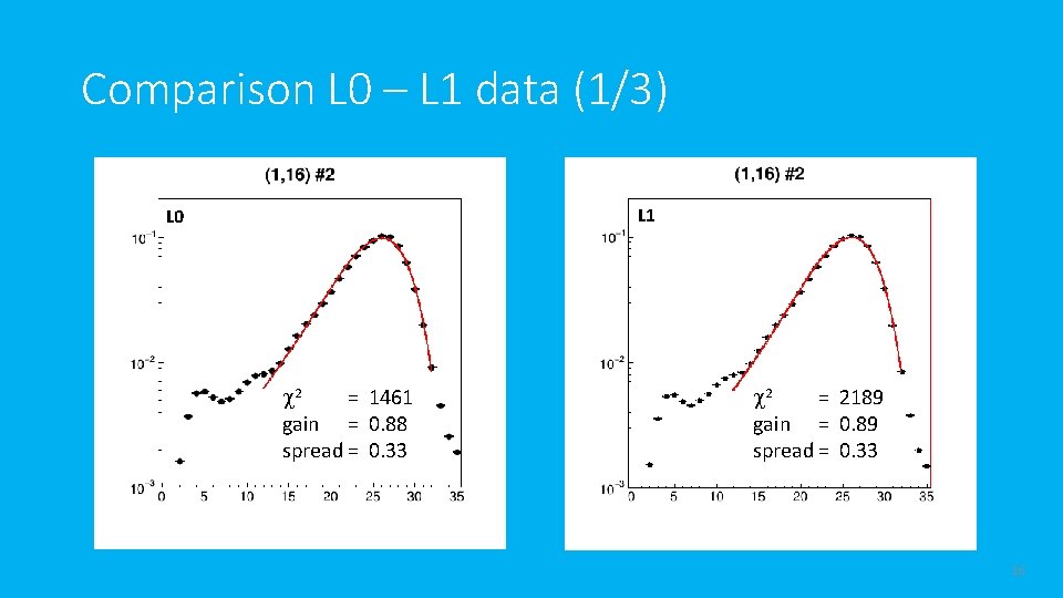
Comparison L 0 – L 1 data (1/3) L 1 L 0 c 2 = 1461 gain = 0. 88 spread = 0. 33 c 2 = 2189 gain = 0. 89 spread = 0. 33 16

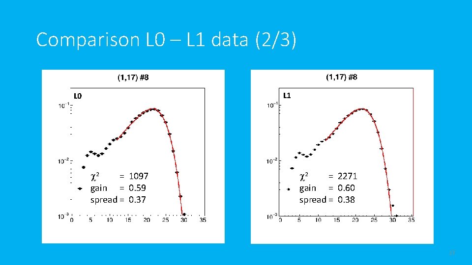
Comparison L 0 – L 1 data (2/3) L 1 L 0 c 2 = 1097 gain = 0. 59 spread = 0. 37 c 2 = 2271 gain = 0. 60 spread = 0. 38 17

Comparison L 0 – L 1 data (3/3) L 1 L 0 c 2 = 1201 gain = 0. 43 spread = 0. 38 c 2 = 3046 gain = 0. 48 spread = 0. 37 18

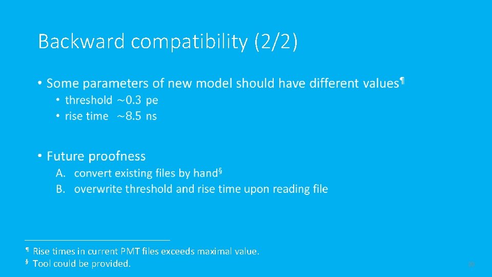
Backward compatibility (1/2) ü New model has less parameters than old model • QE; gain spread; rise time; TTS; threshold; offset; slope; curvature; and saturation ü I/O of model parameters backward compatible (PMT efficiency file) • QE; gain spread; rise time; TTS and threshold 19

Backward compatibility (2/2) • ¶ § Rise times in current PMT files exceeds maximal value. Tool could be provided. 20

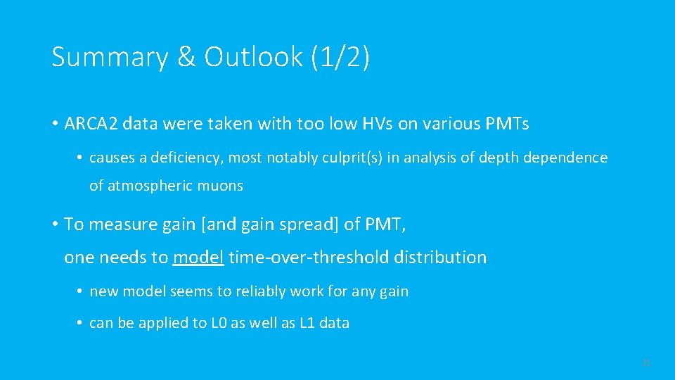
Summary & Outlook (1/2) • ARCA 2 data were taken with too low HVs on various PMTs • causes a deficiency, most notably culprit(s) in analysis of depth dependence of atmospheric muons • To measure gain [and gain spread] of PMT, one needs to model time-over-threshold distribution • new model seems to reliably work for any gain • can be applied to L 0 as well as L 1 data 21

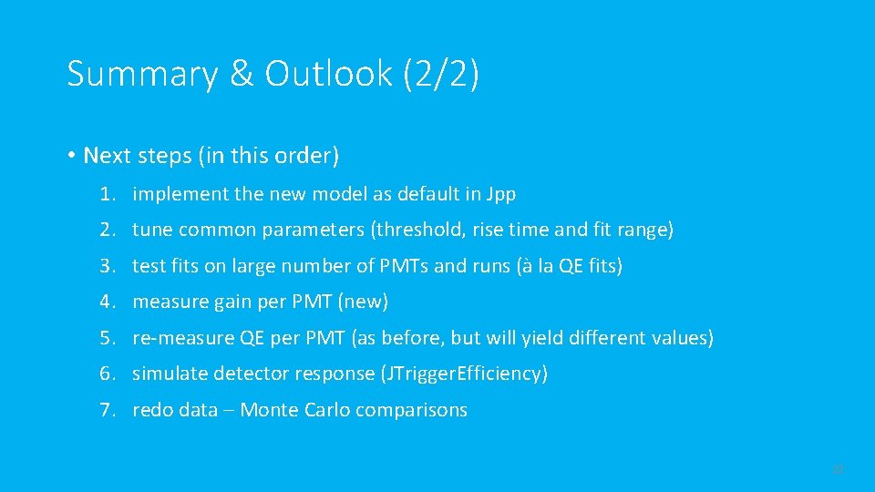
Summary & Outlook (2/2) • Next steps (in this order) 1. implement the new model as default in Jpp 2. tune common parameters (threshold, rise time and fit range) 3. test fits on large number of PMTs and runs (à la QE fits) 4. measure gain per PMT (new) 5. re-measure QE per PMT (as before, but will yield different values) 6. simulate detector response (JTrigger. Efficiency) 7. redo data – Monte Carlo comparisons 22