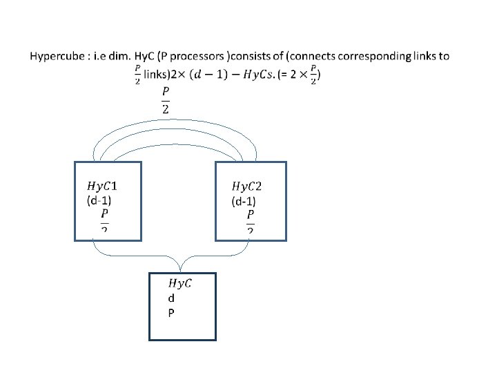
Introduction to Parallel Computing Models of parallel computers


 – for message passing Dynamic (indirect) – for shared")


 - Similar to but - Communication 2 -steps.")


 HC 3")
 HC 3")

 S d")
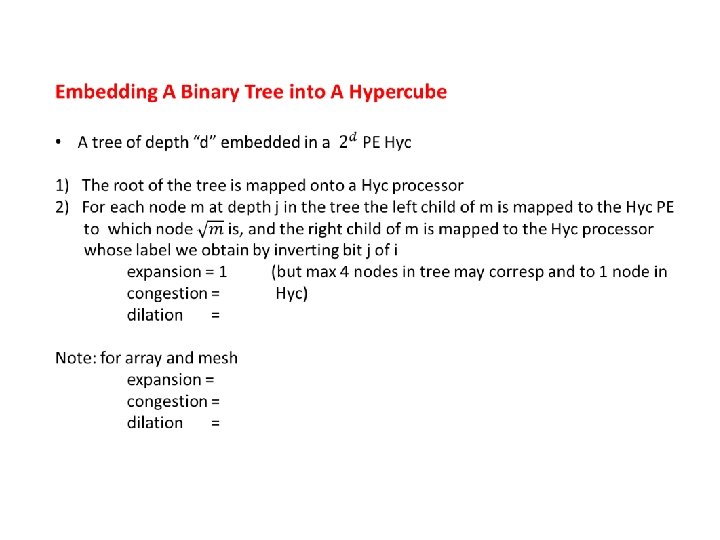
 (b) Fig: A tree rooted at processor 011(=3) and embedded into a threedimensional")


- Slides: 50
Introduction to Parallel Computing
Models of parallel computers: SEQUENTIAL 1. PE M M 2. PE M M
M 3. PE Code M M 4. With Pipelining : f 1 f 2 f 3 f 4 1 M 1 i -------------------------------------2 M 1 i 1 M 2 i -------------------------------------3 M 1 i 2 M 2 i 1 M 3 i
TAXONOMY • • Control Address Space Interconnect. Net. Granularity 1. Control: • SISD – Single Instruction Stream Single Data Stream. - Single program less memory. • SIMD – Single Instruction Stream Multiple Data Stream. - Dedicated hardware (expensive). • MISD – Multiple Instruction Stream Single Data Stream. - Rigid. • MIMD – Multiple Instruction Stream Multiple Data Stream. - program & data all PEs. - Own the self hardware (inexpensive). - flexible
SIMD MIMD global Control Local Control
Address – Space: - Two paradigms: - Message passing - Pain PE + Memory. - Shared Memory - Each PE accesses any location in memory. Message Passing: INN P 1/M P 2/M P/M
Shared Memory: M 1 P 2 P 3 I N N Global Memory Mn Easier to program need specialized hardware(expensive). To minimize communication: Hiding latency technique.
M P NUMA P M Local M m P Local M m I N N Global Memory P Local Memory M P M M I N N
Inter connection Networks: Static (direct) – for message passing Dynamic (indirect) – for shared memory - Fine grain- do not require frequent communication. PRAM- model- (idealized parallel computer. ) P- processor (shave common clock- each works on its own instruction) M- global memory uniformly accessible to all PEs. Synchronous shared- memory computers MIMD. Interaction between PE occurs at no cost.
How is memory accessed by R & W? • • EREW – weakest, minimum concurrency. CREW – write access serialized, read is concurrent. ERCW – write access is concurrent, multiple read access is serialized. CRCW – short powerful – can be simulated on a EREW model. CR – does not need modification in program. CW – access to memory requires arbitration. Protocols: Common – iff all values are identical. Arbitrary – an arbitrary PE proceeds other PEs fail. Priority – PE with highest priority written. Sum – sum of all quantities is written.
Dynamic Inter Connection Networks : i. e. EREW PRAM: – P- Processor m- words in global memory switching elements (Determine the memory word accessed. ) each P can access any of the memory words : -> # member of switching elements Ѳ(mp). (UMA) => expensive => performance Solution: Ø Reduce m try using memory banks (m words organized in b banks) Ø Each P switches between b banks Ø Total # of switching elements Ѳ(bp) Ø Less expensive Note: This is a weak approximate. Of EREW because no 2 PE can access the same memory bank at the same time.
Crossbars Switching Nets M 0 P 1 Pp-1 M 2 Mb-1
Bus-Based Networks Global M BUS UMA
Solution- provide local-cache -> reduces the total # of access to global memory - This implies replicating data => Cache coherency problems Global M BUS Cache
Multistage Interconnection Nets. High # of switching elements Bottle neck Þ Multi stage – provides best trade off. Þ Cost better than CROSS BAR Þ Perf. Better than BUS cost Cross bar Multistage BUS P Perf. Cross bar Multistage BUS P
Multistage Interconnect Net. 6 mega Network: P = # PE B = # memory banks P=b log P = # stages
Model of Parallel Computers
- Switch configuration in one Stage. Pass- through Cross - Over Given by the MSB corresponding to that stage.
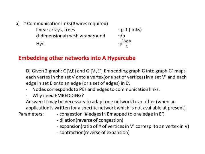
Static Interconnection Nets. - Used in message - passing Completely - Connected Net
Star-Connected Net. - Central PE(bottle neck) - Similar to but - Communication 2 -steps. Linear Array and Ring Linear Array Ring
Tree Net - Only 1 path between any pair of PEs. - Linear arrays and star-connected nets. are special cases of tree nets Static – each node Corresponds to a PE Dynamic – only leaf nodes are Pes - Intermediate nodes are Switching elements S D
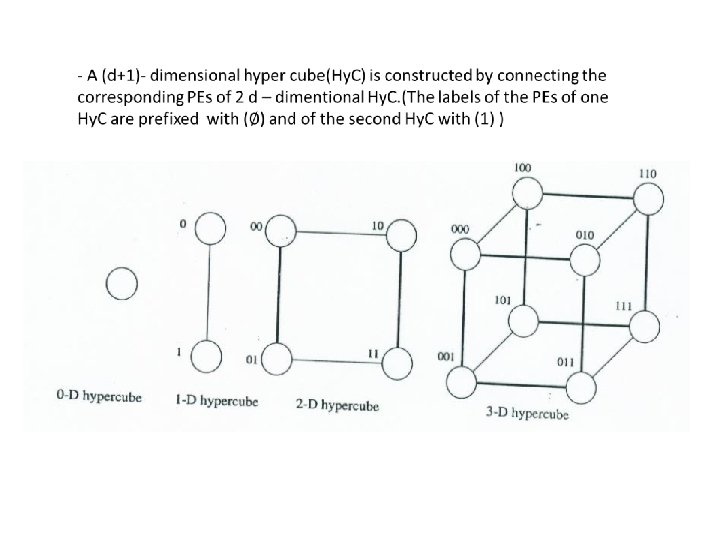
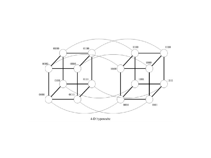
Fat Tree : increasing the number of communication links for PEs closer to the root => In this way bottlenecks at higher levels in the tree are alleviated. 0 -d 1 -d 2 -d 3 -d
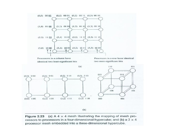
100 000 010 101 001 100 110 Figure HC 2: Three distinct partition of three dimensional hypercube in twodimensional cubes. Link connecting processors within a partition are indicated y bold lines. 010 101 111 011 110 001 111 011 100 000 110 010 101 001 111 011
Fig: b) HC 3
Fig: b) HC 3
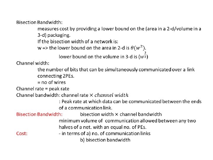
Properties:
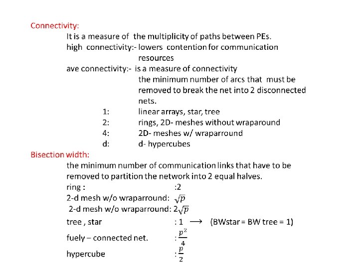
Evaluating static Interconnection Nets (in terms of costs and performance) S d
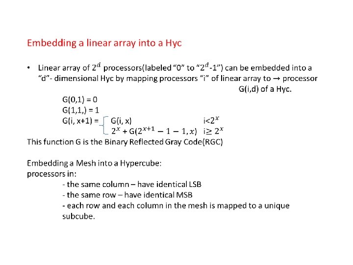
(a) (b) Fig: A tree rooted at processor 011(=3) and embedded into a threedimensional hypercube: a) the organization of the tree rooted at processor 011, and b) the tree embedded into a three-dimensional hypercube.
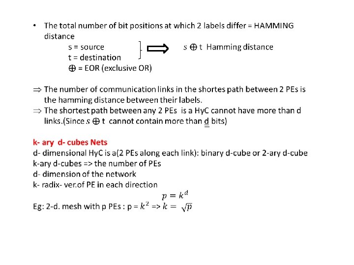
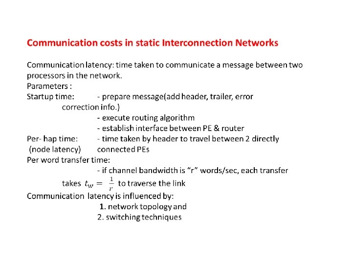
Routing Mechanism for Static Networks Routing mechanism: determines the path a message takes through the network to get from the source to the destination processor. - Considers : - Source - Destination - Info about state of net - Returns one or more path(s) Classification (criteria): -congestion – minimal : (shortest path between source and destination) - does not take in consideration congestion - non minimal: (avoid network congestion)(path may not be shortest) - Use of state of network info – deterministic routing(does not use net. info) - Determines a unique path - Uses only source and destination info. - adaptive (uses network state info. Avoids congestion)
X Y
100 110 Ps 010 Pd 111 000 101 011
time
Cut- through routing store and forward routing: - communication time is high - poor utilization of communication resources Cut through routing: message is advanced from the incoming link to the outgoing link as it arrives - message travels in small units called flow control digits a flits (pipelined through the net) - an intermediate processor does not wait for the entire message to arrive before forwarding it. As soon as flit arrives, it is passed on to the next processor. - all flits are routed along the same path Note: - no need for buffer space to store entire message at intermediate PEs. - uses – less memory (storage) - less memory bandwidth - it is faster
t