Parallel Computing and Parallel Computers ITCS 45145 Cluster

Parallel Computing and Parallel Computers ITCS 4/5145 Cluster Computing, UNC-Charlotte, B. Wilkinson, 2006. 1

Parallel Computing • Using more than one computer, or a computer with more than one processor, to solve a problem. Motives • Usually faster computation - very simple idea - that n computers operating simultaneously can achieve the result n times faster - it will not be n times faster for various reasons. • Other motives include: fault tolerance, larger amount of memory available, . . . 2

Demand for Computational Speed • Continual demand for greater computational speed from a computer system than is currently possible • Areas requiring great computational speed include: – Numerical modeling – Simulation of scientific and engineering problems. • Computations need to be completed within a “reasonable” time period. 3

Grand Challenge Problems Ones that cannot be solved in a reasonable amount of time with today’s computers. Obviously, an execution time of 10 years is always unreasonable. Examples • Modeling large DNA structures • Global weather forecasting • Modeling motion of astronomical bodies. 4

Weather Forecasting • Atmosphere modeled by dividing it into 3 dimensional cells. • Calculations of each cell repeated many times to model passage of time. 5

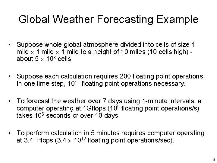
Global Weather Forecasting Example • Suppose whole global atmosphere divided into cells of size 1 mile to a height of 10 miles (10 cells high) about 5 108 cells. • Suppose each calculation requires 200 floating point operations. In one time step, 1011 floating point operations necessary. • To forecast the weather over 7 days using 1 -minute intervals, a computer operating at 1 Gflops (109 floating point operations/s) takes 106 seconds or over 10 days. • To perform calculation in 5 minutes requires computer operating at 3. 4 Tflops (3. 4 1012 floating point operations/sec). 6

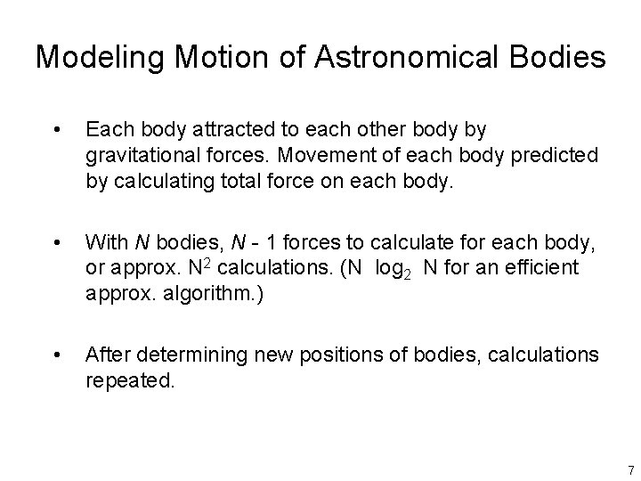
Modeling Motion of Astronomical Bodies • Each body attracted to each other body by gravitational forces. Movement of each body predicted by calculating total force on each body. • With N bodies, N - 1 forces to calculate for each body, or approx. N 2 calculations. (N log 2 N for an efficient approx. algorithm. ) • After determining new positions of bodies, calculations repeated. 7

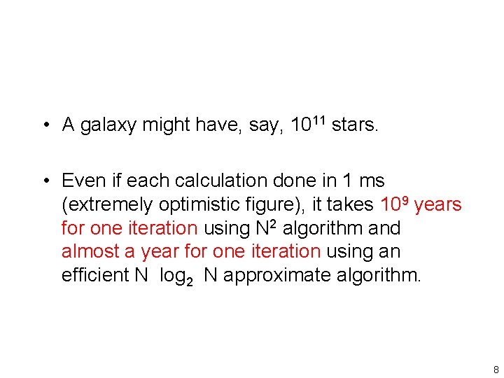
• A galaxy might have, say, 1011 stars. • Even if each calculation done in 1 ms (extremely optimistic figure), it takes 109 years for one iteration using N 2 algorithm and almost a year for one iteration using an efficient N log 2 N approximate algorithm. 8

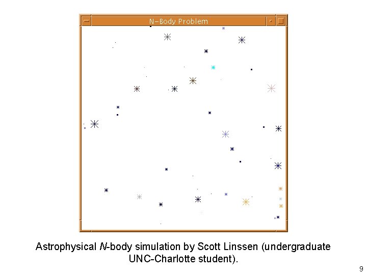
Astrophysical N-body simulation by Scott Linssen (undergraduate UNC-Charlotte student). 9

• Parallel programming – programming parallel computers – Has been around for more than 40 years. 10

Potential for parallel computers/parallel programming 11

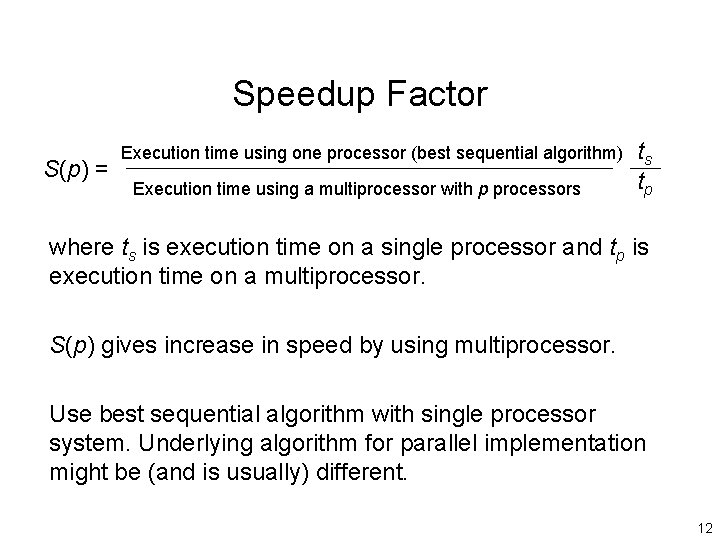
Speedup Factor S(p) = Execution time using one processor (best sequential algorithm) Execution time using a multiprocessor with p processors ts tp where ts is execution time on a single processor and tp is execution time on a multiprocessor. S(p) gives increase in speed by using multiprocessor. Use best sequential algorithm with single processor system. Underlying algorithm for parallel implementation might be (and is usually) different. 12

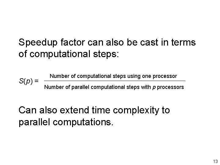
Speedup factor can also be cast in terms of computational steps: S(p) = Number of computational steps using one processor Number of parallel computational steps with p processors Can also extend time complexity to parallel computations. 13

Maximum Speedup Maximum speedup is usually p with p processors (linear speedup). Possible to get superlinear speedup (greater than p) but usually a specific reason such as: • Extra memory in multiprocessor system • Nondeterministic algorithm 14

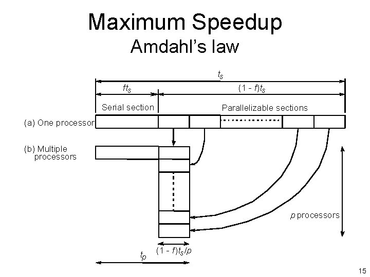
Maximum Speedup Amdahl’s law ts fts (1 - f)ts Serial section Parallelizable sections (a) One processor (b) Multiple processors p processors tp (1 - f)ts /p 15

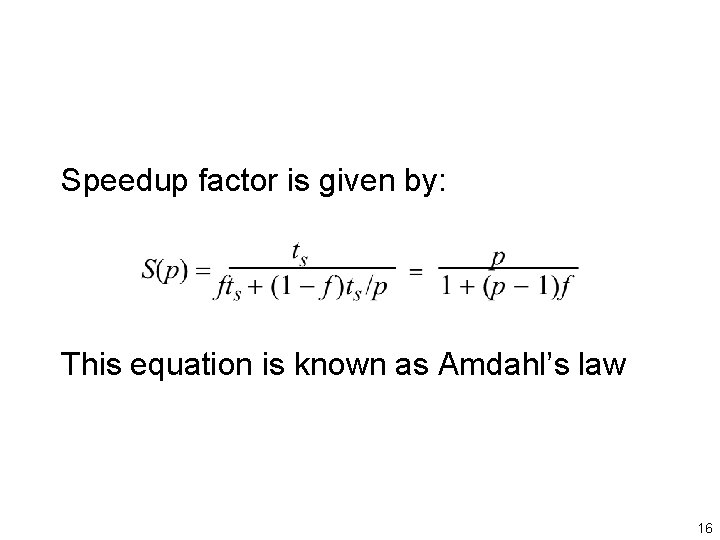
Speedup factor is given by: This equation is known as Amdahl’s law 16

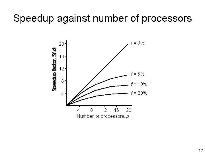
Speedup against number of processors 20 f = 0% 16 12 8 4 f = 5% f = 10% f = 20% 4 8 12 16 20 Number of processors, p 17

Even with infinite number of processors, maximum speedup limited to 1/f. Example With only 5% of computation being serial, maximum speedup is 20, irrespective of number of processors. 18

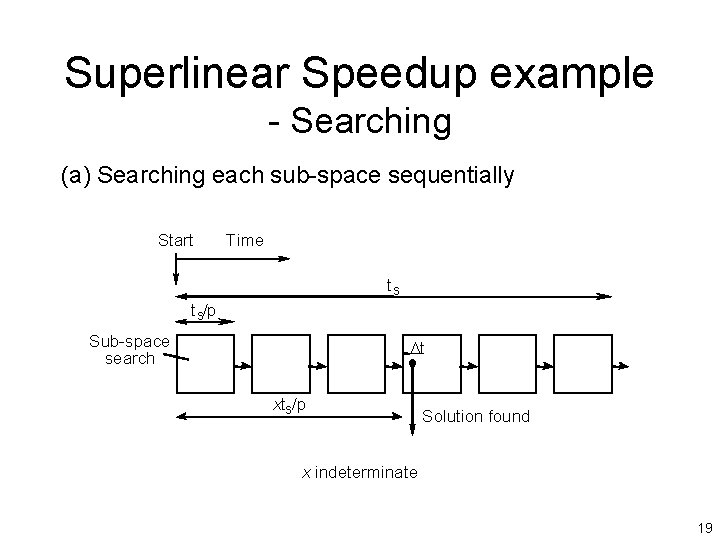
Superlinear Speedup example - Searching (a) Searching each sub-space sequentially Start Time ts t s/p Sub-space search Dt xts/p Solution found x indeterminate 19

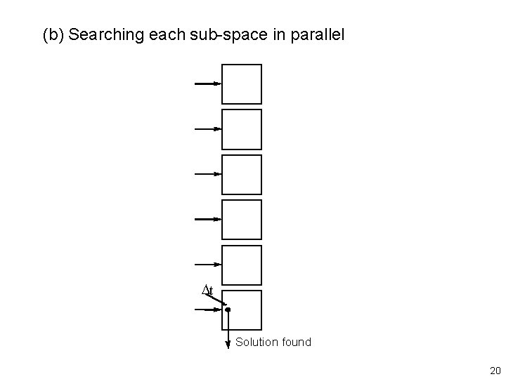
(b) Searching each sub-space in parallel Dt Solution found 20

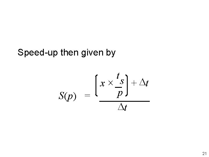
Speed-up then given by x S(p) = ts p Dt + Dt 21

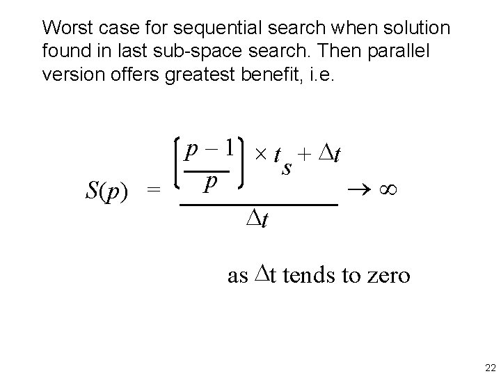
Worst case for sequential search when solution found in last sub-space search. Then parallel version offers greatest benefit, i. e. p – 1 t + Dt s p ®¥ S(p) = Dt as Dt tends to zero 22

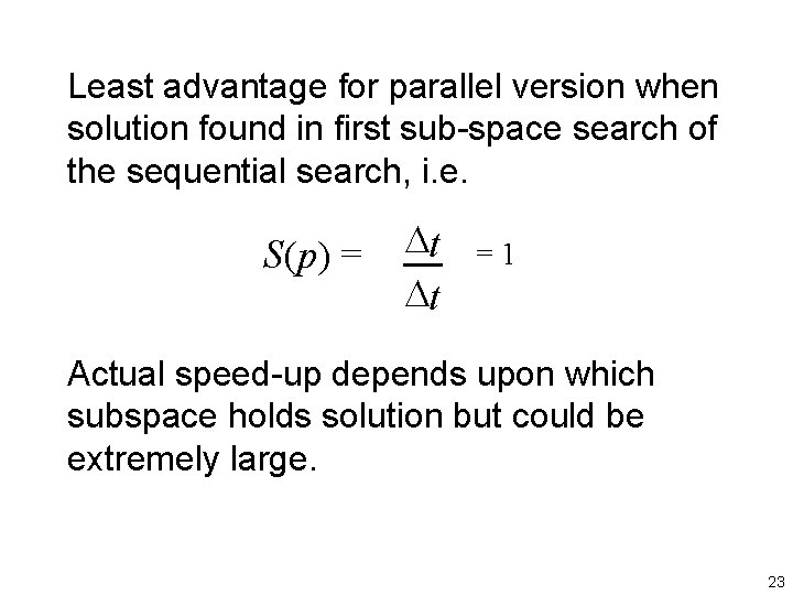
Least advantage for parallel version when solution found in first sub-space search of the sequential search, i. e. S(p) = Dt Dt = 1 Actual speed-up depends upon which subspace holds solution but could be extremely large. 23

• Next question to answer is how does one construct a computer system with multiple processors to achieve the speed-up? 24