Introduction to Artificial Intelligence AI Computer Science cpsc

Introduction to Artificial Intelligence (AI) Computer Science cpsc 502, Lecture 2 Sep, 13, 2011 CPSC 502, Lecture 2 Slide 1

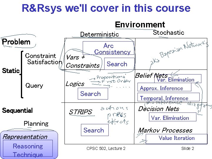
R&Rsys we'll cover in this course Environment Problem Static Deterministic Stochastic Arc Consistency Constraint Vars + Satisfaction Constraints Search Belief Nets Query Logics Search Sequential Planning Representation Reasoning Technique STRIPS Search Var. Elimination Approx. Inference Temporal. Inference Decision Nets Var. Elimination Markov Processes Value Iteration CPSC 502, Lecture 2 Slide 2

Today Sept 13 • • Uninformed Search Informed Search …. …. CPSC 502, Lecture 2 3

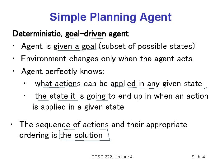
Simple Planning Agent Deterministic, goal-driven agent • Agent is given a goal (subset of possible states) • Environment changes only when the agent acts • Agent perfectly knows: • what actions can be applied in any given state • the state it is going to end up in when an action is applied in a given state • The sequence of actions and their appropriate ordering is the solution CPSC 322, Lecture 4 Slide 4

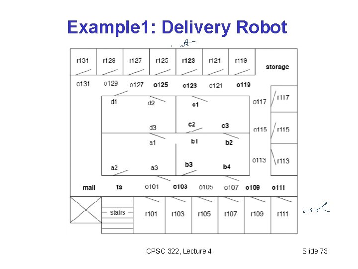
Three examples 1. Solving an 8 -puzzle 2. Vacuum cleaner world 3. A delivery robot planning the route it will take in a bldg. to get from one room to another (see textbook) CPSC 322, Lecture 4 Slide 5

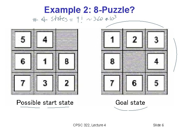
Example 2: 8 -Puzzle? Possible start state CPSC 322, Lecture 4 Goal state Slide 6

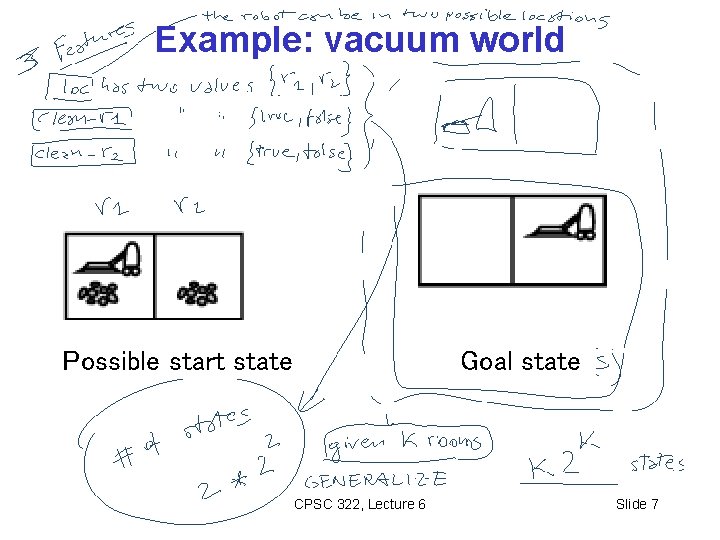
Example: vacuum world Possible start state Goal state CPSC 322, Lecture 6 Slide 7

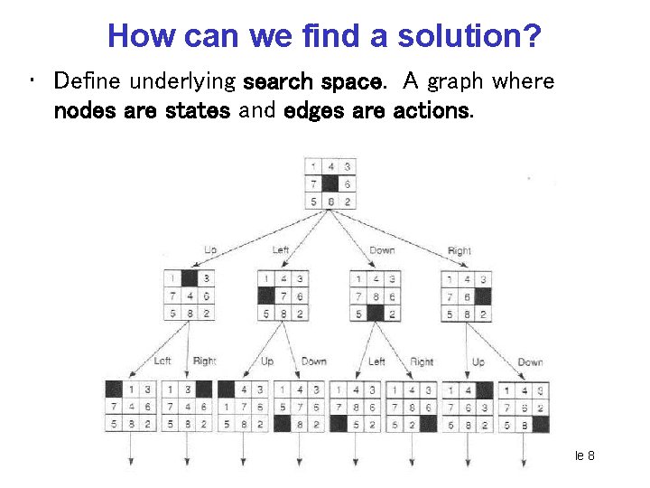
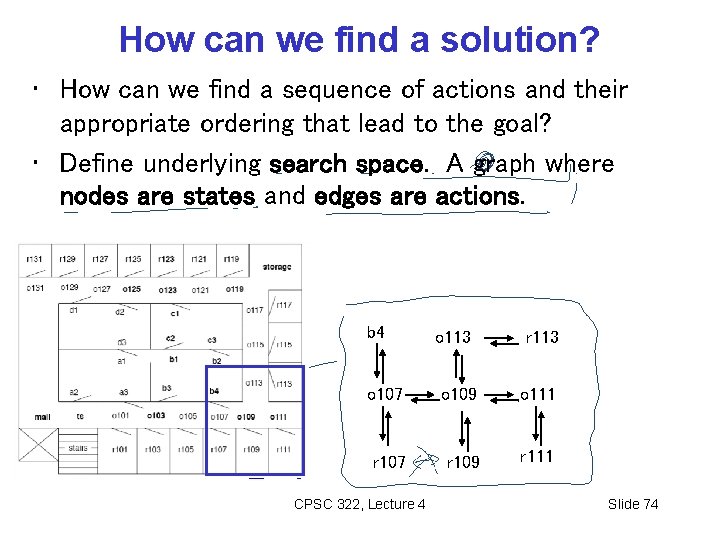
How can we find a solution? • Define underlying search space. A graph where nodes are states and edges are actions. CPSC 322, Lecture 4 Slide 8

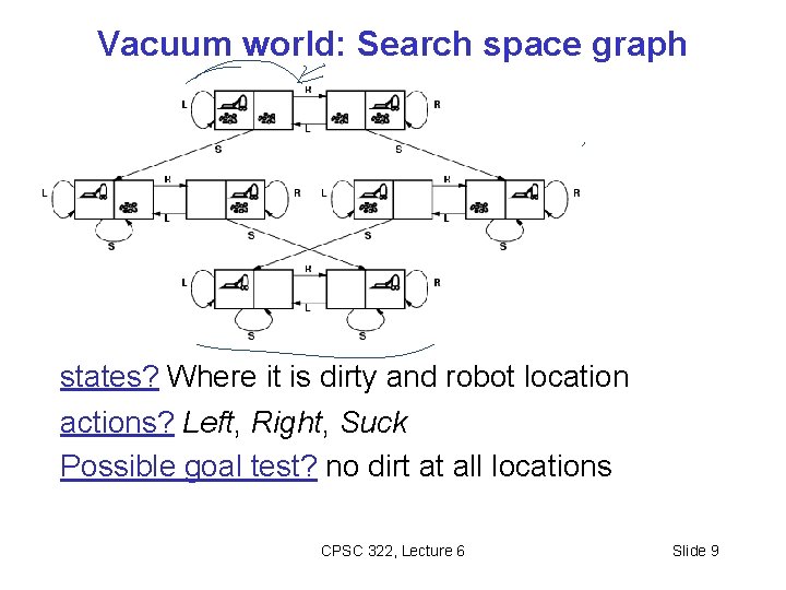
Vacuum world: Search space graph states? Where it is dirty and robot location actions? Left, Right, Suck Possible goal test? no dirt at all locations CPSC 322, Lecture 6 Slide 9

Search: Abstract Definition How to search • Start at the start state • Consider the effect of taking different actions starting from states that have been encountered in the search so far • Stop when a goal state is encountered To make this more formal, we'll need review the formal definition of a graph. . . CPSC 322, Lecture 4 Slide 10

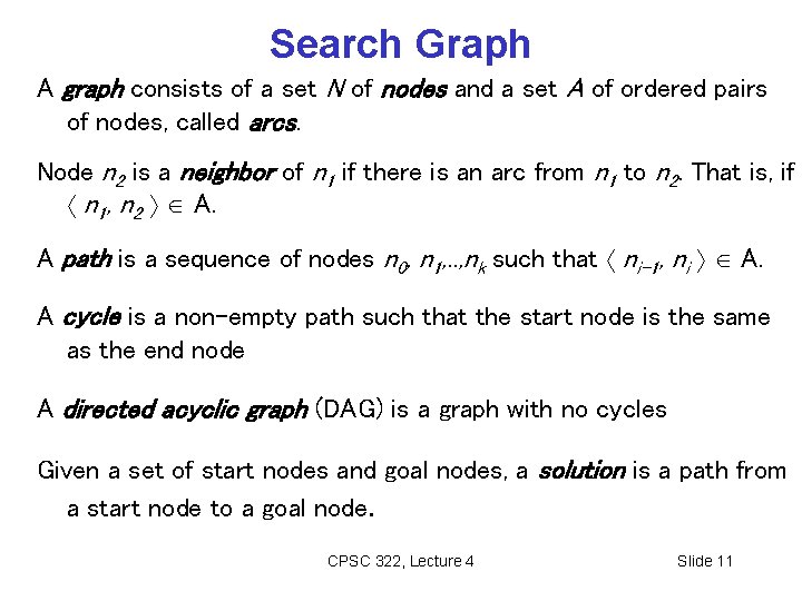
Search Graph A graph consists of a set N of nodes and a set A of ordered pairs of nodes, called arcs. Node n 2 is a neighbor of n 1 if there is an arc from n 1 to n 2. That is, if n 1, n 2 A. A path is a sequence of nodes n 0, n 1, . . , nk such that ni-1, ni A. A cycle is a non-empty path such that the start node is the same as the end node A directed acyclic graph (DAG) is a graph with no cycles Given a set of start nodes and goal nodes, a solution is a path from a start node to a goal node. CPSC 322, Lecture 4 Slide 11

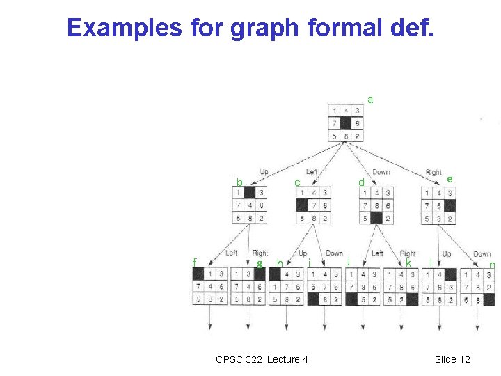
Examples for graph formal def. a b f c g h e d i CPSC 322, Lecture 4 j k l n Slide 12

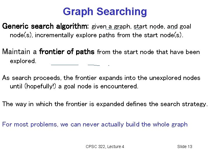
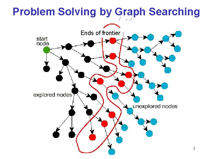
Graph Searching Generic search algorithm: given a graph, start node, and goal node(s), incrementally explore paths from the start node(s). Maintain a frontier of paths from the start node that have been explored. As search proceeds, the frontier expands into the unexplored nodes until (hopefully!) a goal node is encountered. The way in which the frontier is expanded defines the search strategy. For most problems, we can never actually build the whole graph CPSC 322, Lecture 4 Slide 13

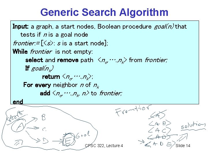
Generic Search Algorithm Input: a graph, a start nodes, Boolean procedure goal(n) that tests if n is a goal node frontier: = [<s>: s is a start node]; While frontier is not empty: select and remove path <no, …. , nk> from frontier; If goal(nk) return <no, …. , nk>; For every neighbor n of nk add <no, …. , nk, n> to frontier; end CPSC 322, Lecture 4 Slide 14

Problem Solving by Graph Searching Ends of frontier CPSC 322, Lecture 4 Slide 15

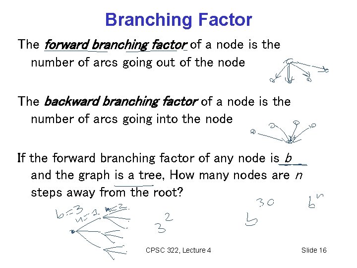
Branching Factor The forward branching factor of a node is the number of arcs going out of the node The backward branching factor of a node is the number of arcs going into the node If the forward branching factor of any node is b and the graph is a tree, How many nodes are n steps away from the root? CPSC 322, Lecture 4 Slide 16

Comparing Searching Algorithms: will it find a solution? the best one? Def. (complete): A search algorithm is complete if, whenever at least one solution exists, the algorithm is guaranteed to find a solution within a finite amount of time. Def. (optimal): A search algorithm is optimal if, when it finds a solution , it is the best solution CPSC 322, Lecture 5 Slide 17

Let’s look at two basic search strategies Depth First and Breath First Search: • To understand key properties of a search strategy • They represent the basis for more sophisticated (heuristic / intelligent) search CPSC 322, Lecture 5 Slide 18

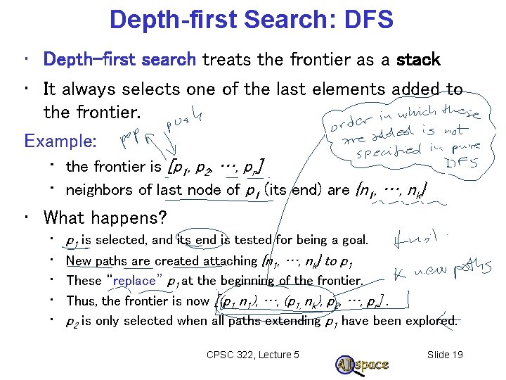
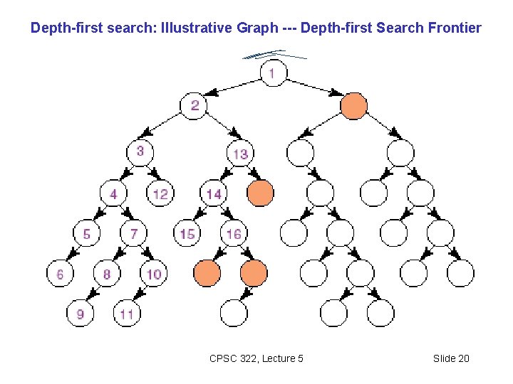
Depth-first Search: DFS • Depth-first search treats the frontier as a stack • It always selects one of the last elements added to the frontier. Example: • the frontier is [p 1, p 2, …, pr] • neighbors of last node of p 1 (its end) are {n 1, …, nk} • What happens? • • • p 1 is selected, and its end is tested for being a goal. New paths are created attaching {n 1, …, nk} to p 1 These “replace” p 1 at the beginning of the frontier. Thus, the frontier is now [(p 1, n 1), …, (p 1, nk), p 2, …, pr]. p 2 is only selected when all paths extending p 1 have been explored. CPSC 322, Lecture 5 Slide 19

Depth-first search: Illustrative Graph --- Depth-first Search Frontier CPSC 322, Lecture 5 Slide 20

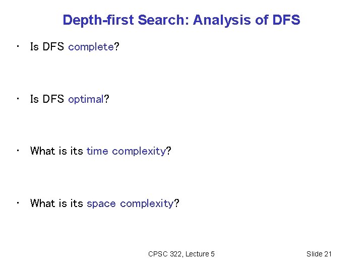
Depth-first Search: Analysis of DFS • Is DFS complete? • Is DFS optimal? • What is its time complexity? • What is its space complexity? CPSC 322, Lecture 5 Slide 21

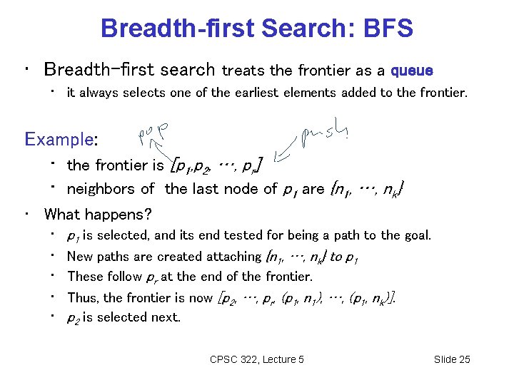
Breadth-first Search: BFS • Breadth-first search treats the frontier as a queue • it always selects one of the earliest elements added to the frontier. Example: • the frontier is [p 1, p 2, …, pr] • neighbors of the last node of p 1 are {n 1, …, nk} • What happens? • p 1 is selected, and its end tested for being a path to the goal. • New paths are created attaching {n 1, …, nk} to p 1 • These follow pr at the end of the frontier. • Thus, the frontier is now [p 2, …, pr, (p 1, n 1), …, (p 1, nk)]. • p 2 is selected next. CPSC 322, Lecture 5 Slide 25

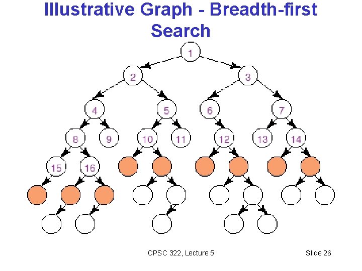
Illustrative Graph - Breadth-first Search CPSC 322, Lecture 5 Slide 26

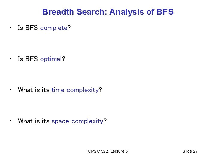
Breadth Search: Analysis of BFS • Is BFS complete? • Is BFS optimal? • What is its time complexity? • What is its space complexity? CPSC 322, Lecture 5 Slide 27

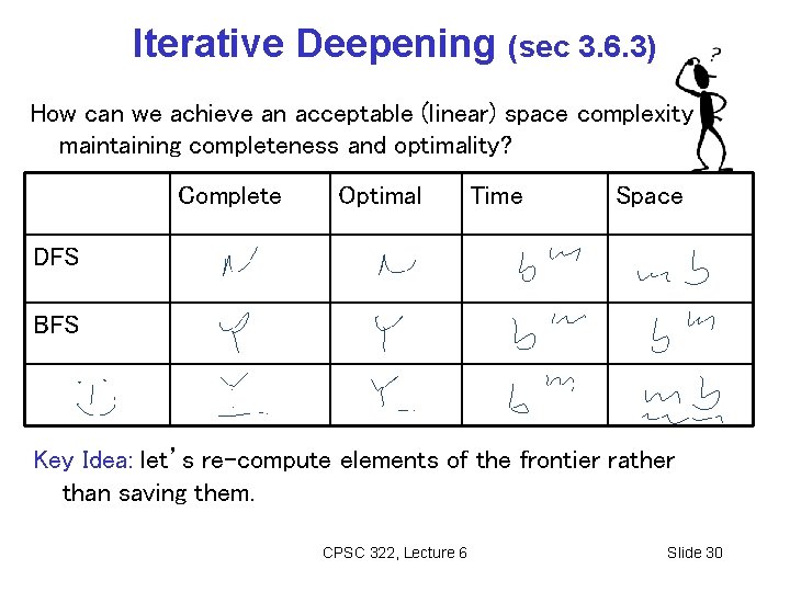
Iterative Deepening (sec 3. 6. 3) How can we achieve an acceptable (linear) space complexity maintaining completeness and optimality? Complete Optimal Time Space DFS BFS Key Idea: let’s re-compute elements of the frontier rather than saving them. CPSC 322, Lecture 6 Slide 30

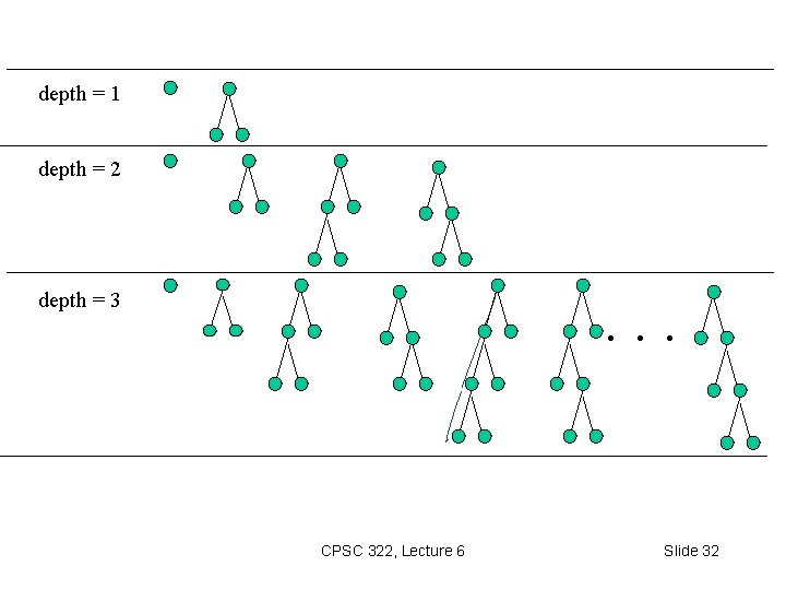
Iterative Deepening in Essence • Look with DFS for solutions at depth 1, then 2, then 3, etc. • If a solution cannot be found at depth D, look for a solution at depth D + 1. • You need a depth-bounded depth-first searcher. • Given a bound B you simply assume that paths of length B cannot be expanded…. CPSC 322, Lecture 6 Slide 31

depth = 1 depth = 2 depth = 3 . . . CPSC 322, Lecture 6 Slide 32

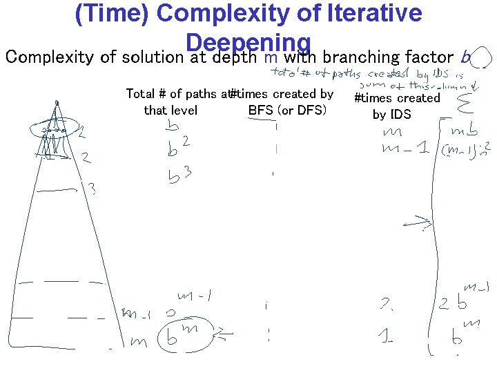
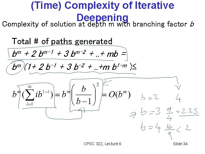
(Time) Complexity of Iterative Deepening Complexity of solution at depth m with branching factor b Total # of paths at#times created by that level BFS (or DFS) #times created by IDS

(Time) Complexity of Iterative Deepening Complexity of solution at depth m with branching factor b Total # of paths generated bm + 2 bm-1 + 3 bm-2 +. . + mb = bm (1+ 2 b-1 + 3 b-2 +. . +m b 1 -m )≤ CPSC 322, Lecture 6 Slide 34

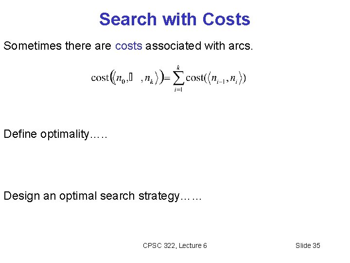
Search with Costs Sometimes there are costs associated with arcs. Define optimality…. . Design an optimal search strategy…… CPSC 322, Lecture 6 Slide 35

Today Sept 13 • • Uninformed Search Informed Search …. …. CPSC 502, Lecture 2 36

Heuristic Search Uninformed/Blind search algorithms do not take into account the goal until they are at a goal node. Often there is extra knowledge that can be used to guide the search: an estimate of the distance from node n to a goal node. This is called a heuristic CPSC 322, Lecture 7 Slide 37

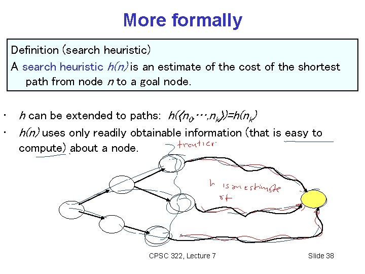
More formally Definition (search heuristic) A search heuristic h(n) is an estimate of the cost of the shortest path from node n to a goal node. • • h can be extended to paths: h( n 0, …, nk )=h(nk) h(n) uses only readily obtainable information (that is easy to compute) about a node. CPSC 322, Lecture 7 Slide 38

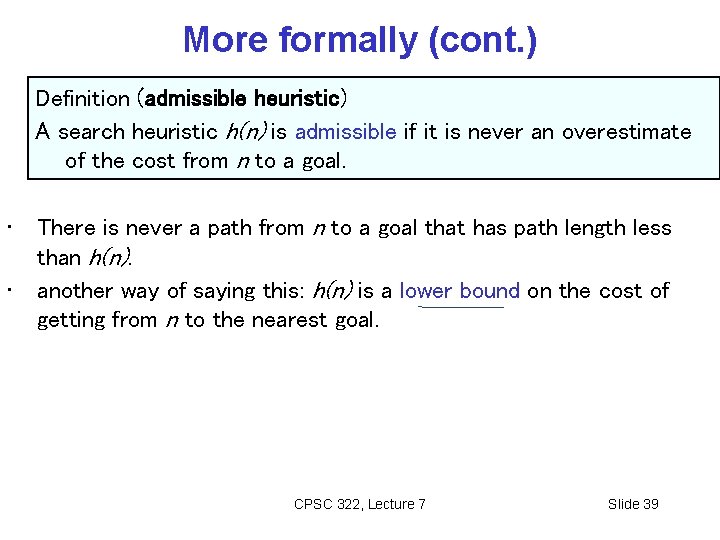
More formally (cont. ) Definition (admissible heuristic) A search heuristic h(n) is admissible if it is never an overestimate of the cost from n to a goal. • • There is never a path from n to a goal that has path length less than h(n). another way of saying this: h(n) is a lower bound on the cost of getting from n to the nearest goal. CPSC 322, Lecture 7 Slide 39

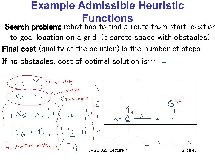
Example Admissible Heuristic Functions Search problem: robot has to find a route from start location to goal location on a grid (discrete space with obstacles) Final cost (quality of the solution) is the number of steps If no obstacles, cost of optimal solution is… CPSC 322, Lecture 7 Slide 40

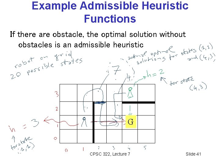
Example Admissible Heuristic Functions If there are obstacle, the optimal solution without obstacles is an admissible heuristic G CPSC 322, Lecture 7 Slide 41

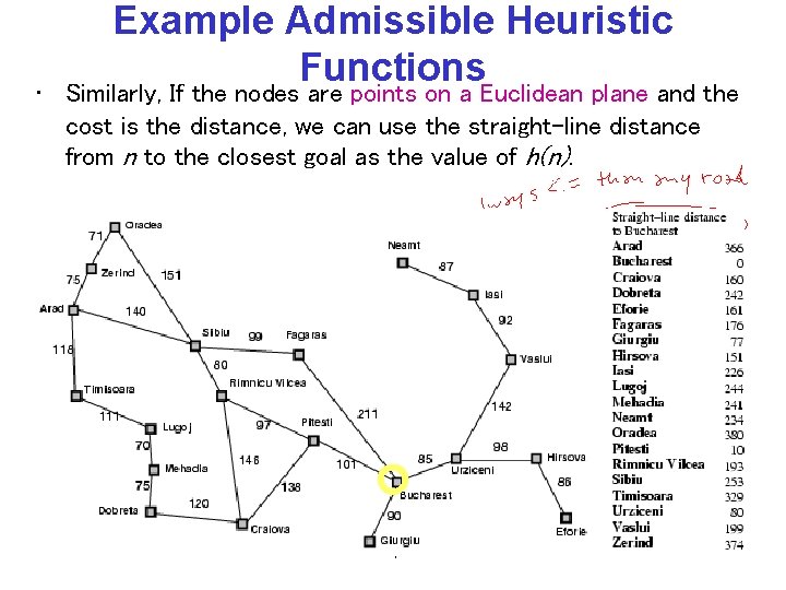
Example Admissible Heuristic Functions • Similarly, If the nodes are points on a Euclidean plane and the cost is the distance, we can use the straight-line distance from n to the closest goal as the value of h(n). CPSC 322, Lecture 7 Slide 42

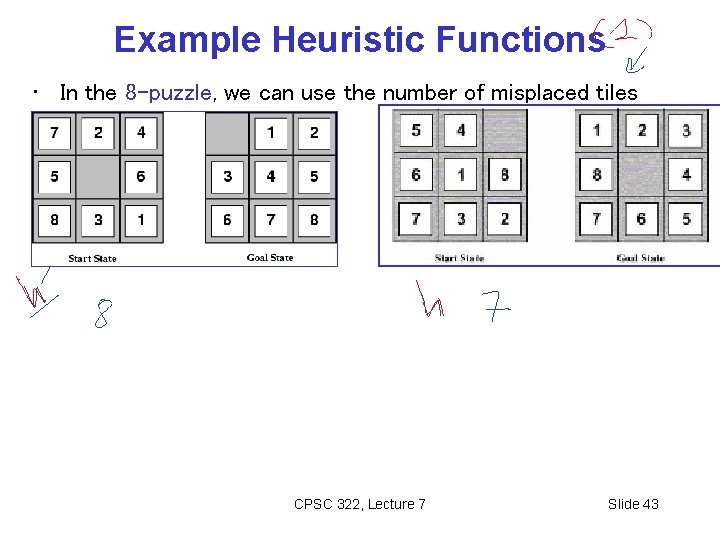
Example Heuristic Functions • In the 8 -puzzle, we can use the number of misplaced tiles CPSC 322, Lecture 7 Slide 43

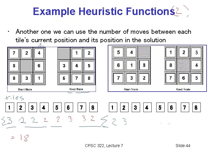
Example Heuristic Functions • Another one we can use the number of moves between each tile's current position and its position in the solution 1 2 3 4 5 6 7 8 1 2 CPSC 322, Lecture 7 3 4 5 6 7 Slide 44 8

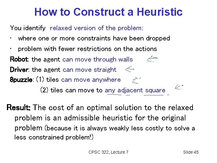
How to Construct a Heuristic You identify relaxed version of the problem: • where one or more constraints have been dropped • problem with fewer restrictions on the actions Robot: the agent can move through walls Driver: the agent can move straight 8 puzzle: (1) tiles can move anywhere (2) tiles can move to any adjacent square Result: The cost of an optimal solution to the relaxed problem is an admissible heuristic for the original problem (because it is always weakly less costly to solve a less constrained problem!) CPSC 322, Lecture 7 Slide 45

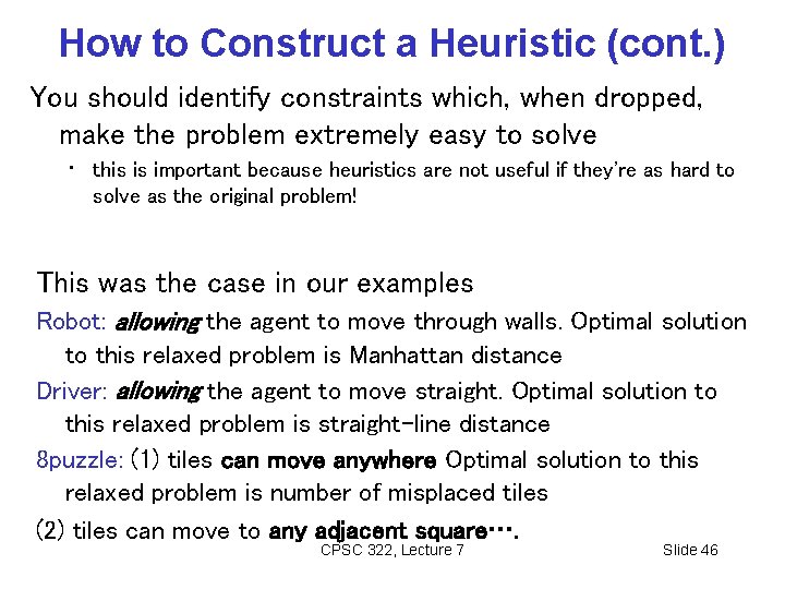
How to Construct a Heuristic (cont. ) You should identify constraints which, when dropped, make the problem extremely easy to solve • this is important because heuristics are not useful if they're as hard to solve as the original problem! This was the case in our examples Robot: allowing the agent to move through walls. Optimal solution to this relaxed problem is Manhattan distance Driver: allowing the agent to move straight. Optimal solution to this relaxed problem is straight-line distance 8 puzzle: (1) tiles can move anywhere Optimal solution to this relaxed problem is number of misplaced tiles (2) tiles can move to any adjacent square…. CPSC 322, Lecture 7 Slide 46

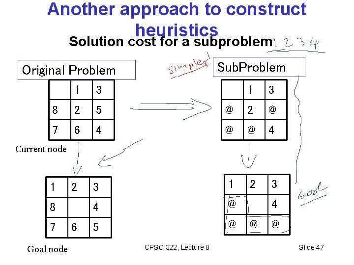
Another approach to construct heuristics Solution cost for a subproblem Sub. Problem Original Problem 1 3 8 2 5 @ 2 @ 7 6 4 @ @ 4 2 3 1 2 3 4 @ 5 @ Current node 1 8 7 Goal node 6 CPSC 322, Lecture 8 4 @ @ Slide 47

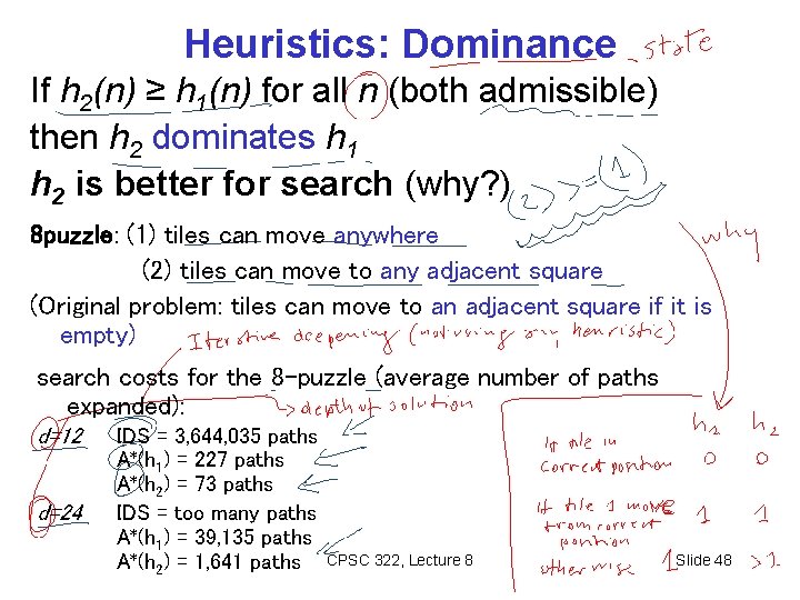
Heuristics: Dominance If h 2(n) ≥ h 1(n) for all n (both admissible) then h 2 dominates h 1 h 2 is better for search (why? ) 8 puzzle: (1) tiles can move anywhere (2) tiles can move to any adjacent square (Original problem: tiles can move to an adjacent square if it is empty) search costs for the 8 -puzzle (average number of paths expanded): d=12 d=24 IDS = 3, 644, 035 paths A*(h 1) = 227 paths A*(h 2) = 73 paths IDS = too many paths A*(h 1) = 39, 135 paths A*(h 2) = 1, 641 paths CPSC 322, Lecture 8 Slide 48

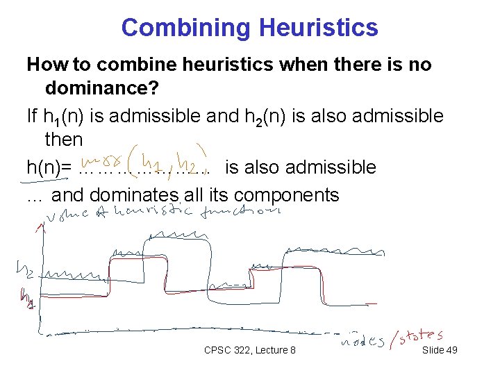
Combining Heuristics How to combine heuristics when there is no dominance? If h 1(n) is admissible and h 2(n) is also admissible then h(n)= ………………… is also admissible … and dominates all its components CPSC 322, Lecture 8 Slide 49

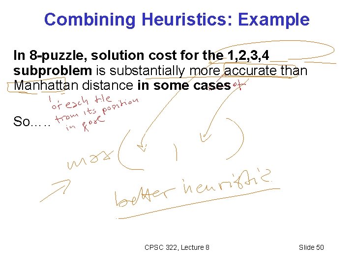
Combining Heuristics: Example In 8 -puzzle, solution cost for the 1, 2, 3, 4 subproblem is substantially more accurate than Manhattan distance in some cases So…. . CPSC 322, Lecture 8 Slide 50

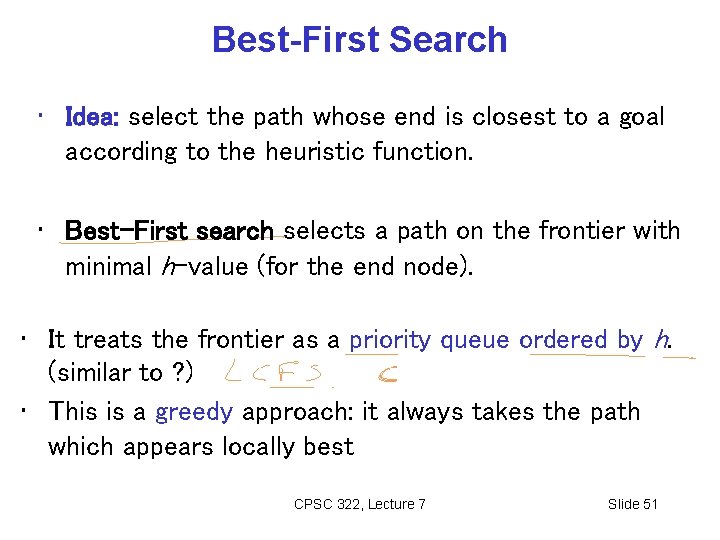
Best-First Search • Idea: select the path whose end is closest to a goal according to the heuristic function. • Best-First search selects a path on the frontier with minimal h-value (for the end node). • It treats the frontier as a priority queue ordered by h. (similar to ? ) • This is a greedy approach: it always takes the path which appears locally best CPSC 322, Lecture 7 Slide 51

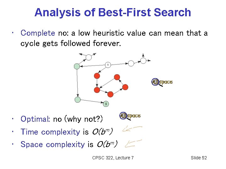
Analysis of Best-First Search • Complete no: a low heuristic value can mean that a cycle gets followed forever. • Optimal: no (why not? ) • Time complexity is O(bm) • Space complexity is O(bm) CPSC 322, Lecture 7 Slide 52

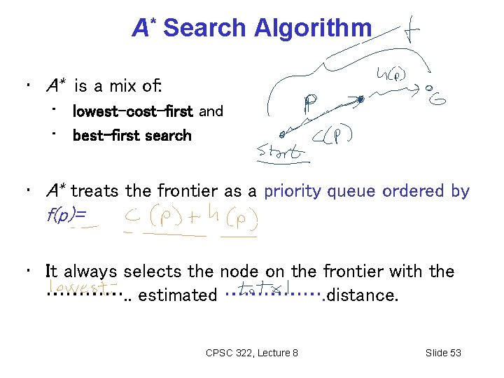
A* Search Algorithm • A* is a mix of: • lowest-cost-first and • best-first search • A* treats the frontier as a priority queue ordered by f(p)= • It always selects the node on the frontier with the …………. . estimated ……………. distance. CPSC 322, Lecture 8 Slide 53

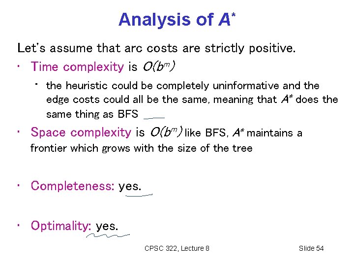
Analysis of A* Let's assume that arc costs are strictly positive. • Time complexity is O(bm) • the heuristic could be completely uninformative and the edge costs could all be the same, meaning that A* does the same thing as BFS • Space complexity is O(bm) like BFS, A* maintains a frontier which grows with the size of the tree • Completeness: yes. • Optimality: yes. CPSC 322, Lecture 8 Slide 54

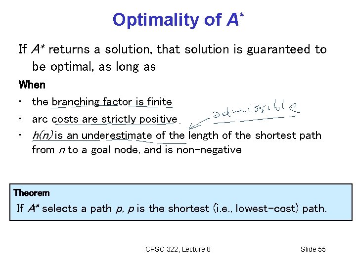
Optimality of A* If A* returns a solution, that solution is guaranteed to be optimal, as long as When • the branching factor is finite • arc costs are strictly positive • h(n) is an underestimate of the length of the shortest path from n to a goal node, and is non-negative Theorem If A* selects a path p, p is the shortest (i. e. , lowest-cost) path. CPSC 322, Lecture 8 Slide 55

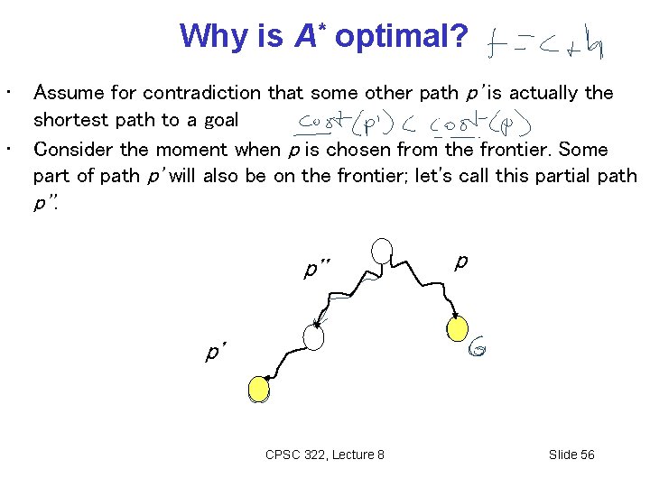
Why is A* optimal? • • Assume for contradiction that some other path p' is actually the shortest path to a goal Consider the moment when p is chosen from the frontier. Some part of path p' will also be on the frontier; let's call this partial path p'' p p' CPSC 322, Lecture 8 Slide 56

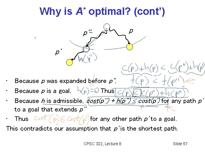
Why is A* optimal? (cont’) p'' p p' Because p was expanded before p'', Because p is a goal, Thus Because h is admissible, cost(p'') + h(p'') cost(p') for any path p' to a goal that extends p'' • Thus for any other path p' to a goal. This contradicts our assumption that p' is the shortest path. • • • CPSC 322, Lecture 8 Slide 57

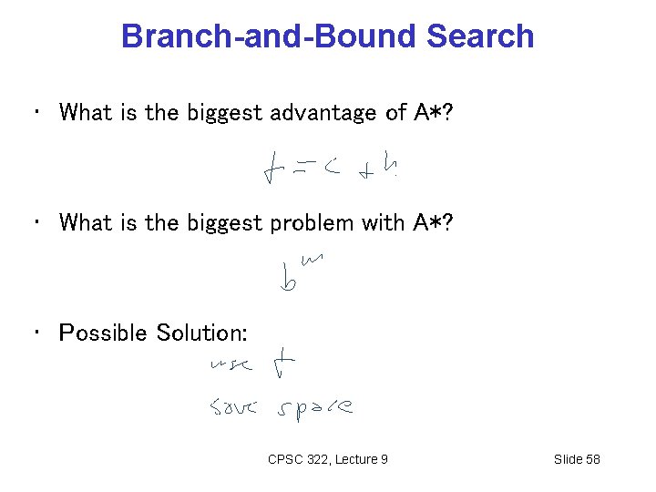
Branch-and-Bound Search • What is the biggest advantage of A*? • What is the biggest problem with A*? • Possible Solution: CPSC 322, Lecture 9 Slide 58

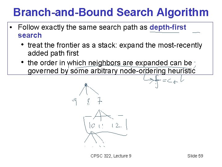
Branch-and-Bound Search Algorithm • Follow exactly the same search path as depth-first search • treat the frontier as a stack: expand the most-recently added path first • the order in which neighbors are expanded can be governed by some arbitrary node-ordering heuristic CPSC 322, Lecture 9 Slide 59

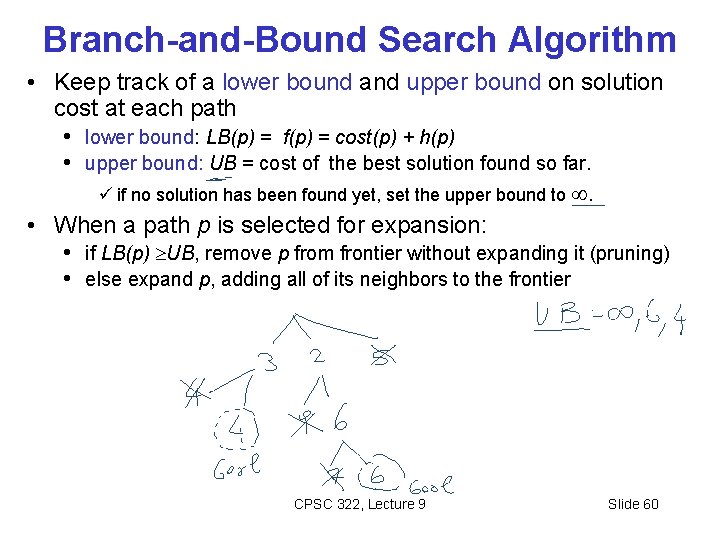
Branch-and-Bound Search Algorithm • Keep track of a lower bound and upper bound on solution cost at each path • lower bound: LB(p) = f(p) = cost(p) + h(p) • upper bound: UB = cost of the best solution found so far. ü if no solution has been found yet, set the upper bound to . • When a path p is selected for expansion: • if LB(p) UB, remove p from frontier without expanding it (pruning) • else expand p, adding all of its neighbors to the frontier CPSC 322, Lecture 9 Slide 60

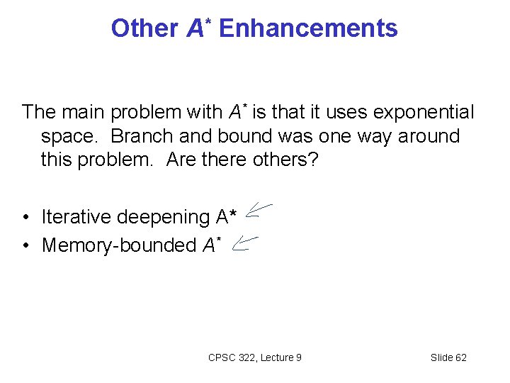
Other A* Enhancements The main problem with A* is that it uses exponential space. Branch and bound was one way around this problem. Are there others? • Iterative deepening A* • Memory-bounded A* CPSC 322, Lecture 9 Slide 62

Other A* Enhancements The main problem with A* is that it uses exponential space. Branch and bound was one way around this problem. Are there others? • Iterative deepening A* • Memory-bounded A* CPSC 322, Lecture 9 Slide 63

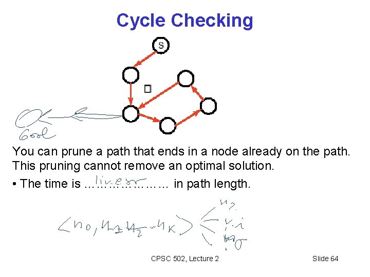
Cycle Checking You can prune a path that ends in a node already on the path. This pruning cannot remove an optimal solution. • The time is ………………… in path length. CPSC 502, Lecture 2 Slide 64

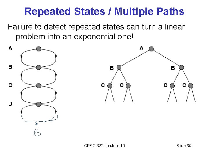
Repeated States / Multiple Paths Failure to detect repeated states can turn a linear problem into an exponential one! CPSC 322, Lecture 10 Slide 65

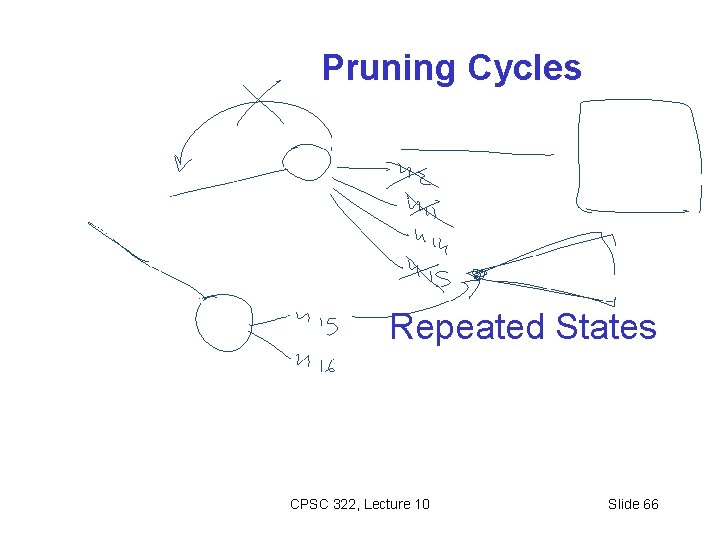
Pruning Cycles Repeated States CPSC 322, Lecture 10 Slide 66

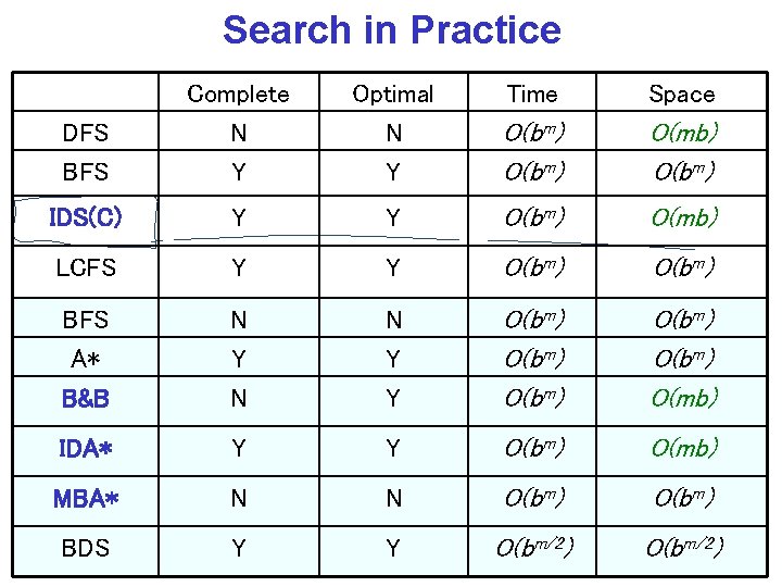
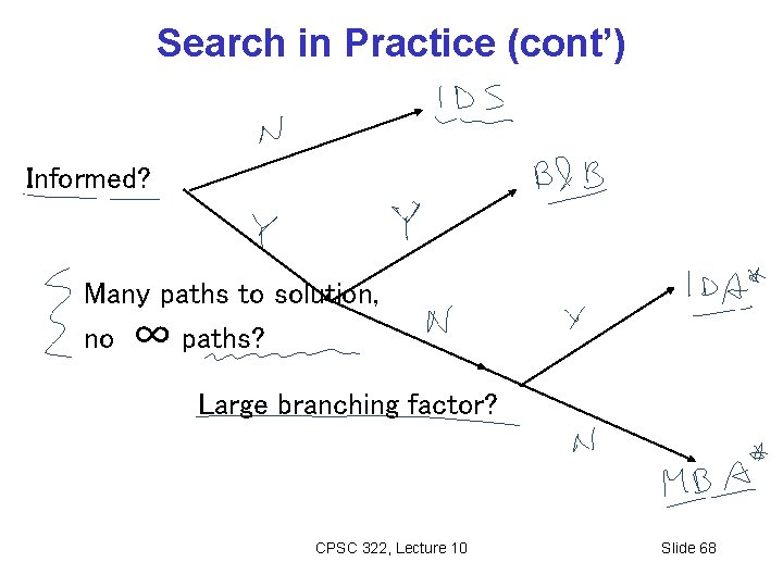
Search in Practice Optimal N Y Time Space DFS BFS Complete N Y O(bm) O(mb) O(bm) IDS(C) Y Y O(bm) O(mb) LCFS Y Y O(bm) BFS A* B&B N Y N N Y Y O(bm) O(bm) O(mb) IDA* Y Y O(bm) O(mb) MBA* N N O(bm) BDS Y CPSC 322, Lecture 10 Y O(bm/2) m/2 Slide 67) O(b

Search in Practice (cont’) Informed? Many paths to solution, no ∞ paths? Large branching factor? CPSC 322, Lecture 10 Slide 68

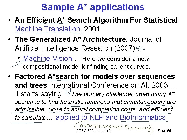
Sample A* applications • An Efficient A* Search Algorithm For Statistical Machine Translation. 2001 • The Generalized A* Architecture. Journal of Artificial Intelligence Research (2007) • Machine Vision … Here we consider a new compositional model for finding salient curves. • Factored A*search for models over sequences and trees International Conference on AI. 2003…. It starts saying… The primary challenge when using A* search is to find heuristic functions that simultaneously are admissible, close to actual completion costs, and efficient to calculate… applied to NLP and Bio. Informatics CPSC 322, Lecture 9 Slide 69

Class Forum: Piazza Join the class asap via the signup link below. http: //www. piazza. com/ubc. ca/fall 2011/cpsc 5 02 You need a ubc. ca or cs. ubc. ca email address to sign up. If you do not have one, please send an email to rjoty@cs. ubc. ca CPSC 502, Lecture 2 Slide 70

TODO for this Thurs Read Chp 4 of textbook Do all the “Graph Searching exercises” available at http: //www. aispace. org/exercises. shtml Please, look at solutions only after you have tried hard to solve them! • Join piazza (the class discussion forum) CPSC 502, Lecture 2 Slide 71

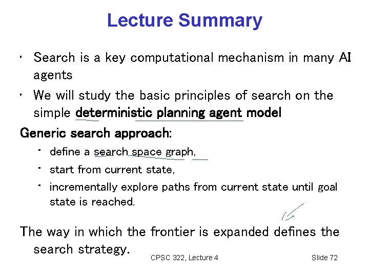
Lecture Summary • Search is a key computational mechanism in many AI agents • We will study the basic principles of search on the simple deterministic planning agent model Generic search approach: • define a search space graph, • start from current state, • incrementally explore paths from current state until goal state is reached. The way in which the frontier is expanded defines the search strategy. CPSC 322, Lecture 4 Slide 72

Example 1: Delivery Robot CPSC 322, Lecture 4 Slide 73

How can we find a solution? • How can we find a sequence of actions and their appropriate ordering that lead to the goal? • Define underlying search space. A graph where nodes are states and edges are actions. b 4 o 113 r 113 o 107 o 109 o 111 r 107 r 109 r 111 CPSC 322, Lecture 4 Slide 74

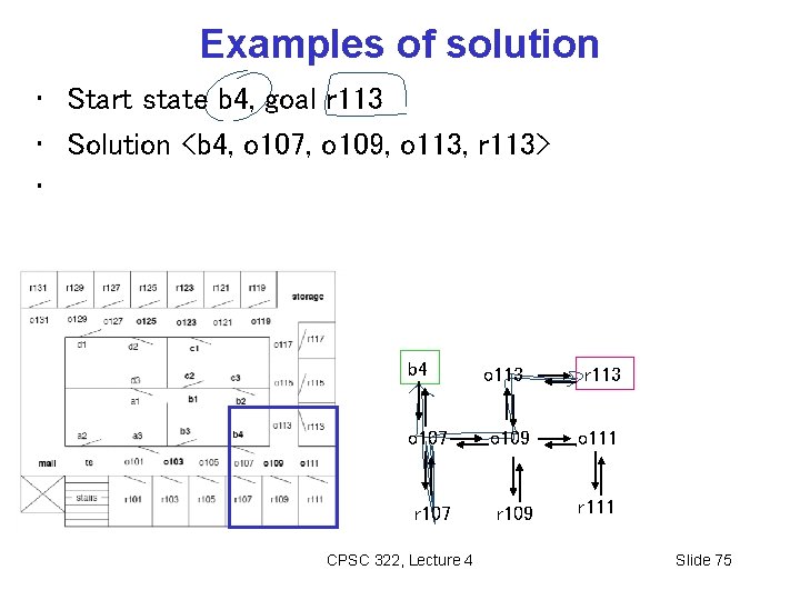
Examples of solution • Start state b 4, goal r 113 • Solution <b 4, o 107, o 109, o 113, r 113> • b 4 o 113 r 113 o 107 o 109 o 111 r 107 r 109 r 111 CPSC 322, Lecture 4 Slide 75